

Reinforcement Learning · Lecture 1
Exploration Methods
Rafael Fernandes Cunha
Welcome!
Rafael F. Cunha
Lecturer @ Leiden University
Ph.D. Candidate @ University of Groningen
Research topics:
•Multiagent RL
•Transfer Learning in RL
•RL-based Post-training of LLMs with Analytic/Verifiable
Rewards
MSc. in Systems and Control.
BSc. in Electronic Engineering.
Hobbies: Biking in the countryside.

Course Material
•Main Material
•Book Reinforcement Learning: An Introduction
•Freely available at the authors website:
http://incompleteideas.net/book/the-book-2nd.html
•Other Materials
•UCL x Deepmind RL Lecture Series:
https://www.youtube.com/playlist?list=PLqYmG7hTraZCRwoyGxv
QkqVrZgDQi4m-5
•Lecture notes from the course CSCI 531 from the St. Francis
Xavier university. https://people.stfx.ca/jdelamer/courses/csci-
531/index.html
•Gymnasium, a library with many environments to evaluate the RL
algorithms: https://gymnasium.farama.org/
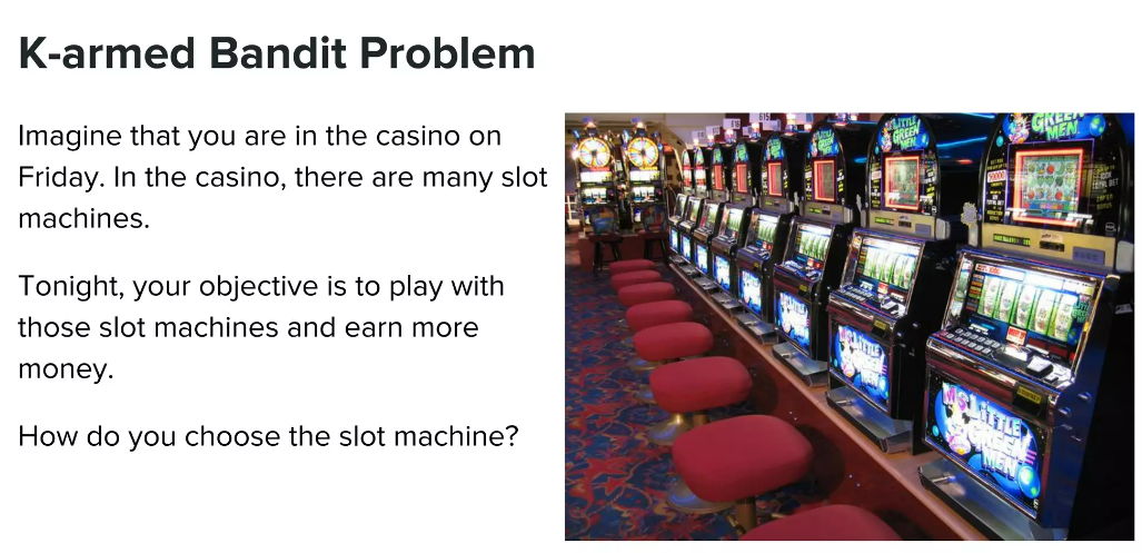
The multi-armed bandit problem
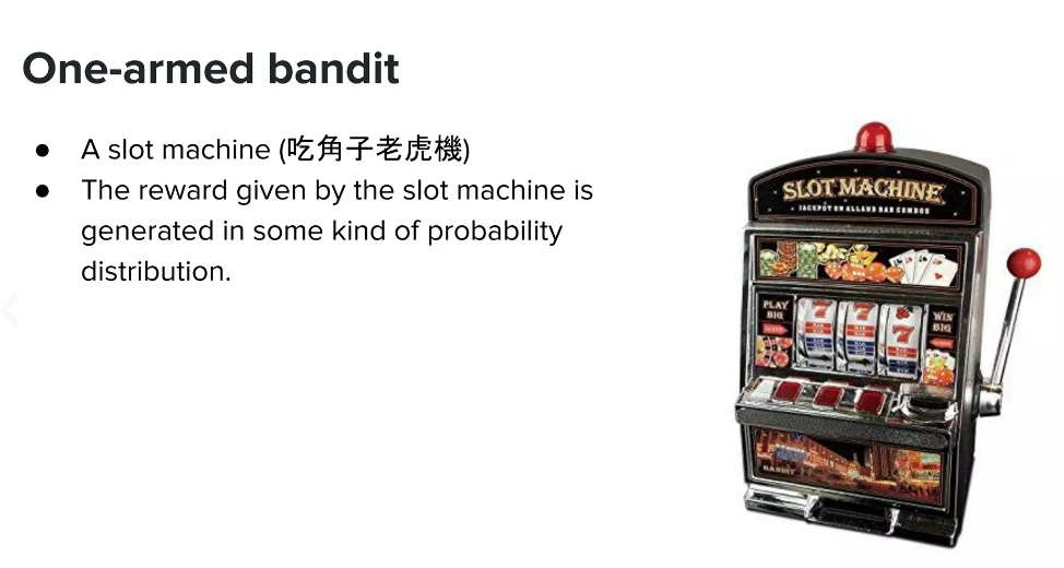
•You are in a casino with many slot machines.
•You will play 1000 times.
•Each time, you choose one machine.
•Your goal is to win as much money as possible.
How do you choose which slot
machine to play each time?
What do we know about these slot machines?
Consider the 1st slot machine.
You pull its arm 5 times and observe
the following payouts (rewards ).
= 2
= 1
= -1
= 3
= 0
Why are we receiving
different rewards if the
machine is the same?
Which mathematical concept are we talking about here? [Review]
1
Random variables (RVs)
•RVs are the staple of probability & statistics
Do you know what a random variable is?
It’s a variable whose value is unknown, not fixed, but dependent upon chance.
«Which is the area of a triangle
given that the base is 12cm and
the height is 14cm?»
Conventional
variable: its value
is fixed once we
define and
«How tall is a random man from
the Netherlands?»
«I am going to flip a fair coin.
Which is the result?»


Height of Jan
Result of coin
Random
variables
[Review]
Two Flavors of RV: Discrete vs. Continuous
[Review]
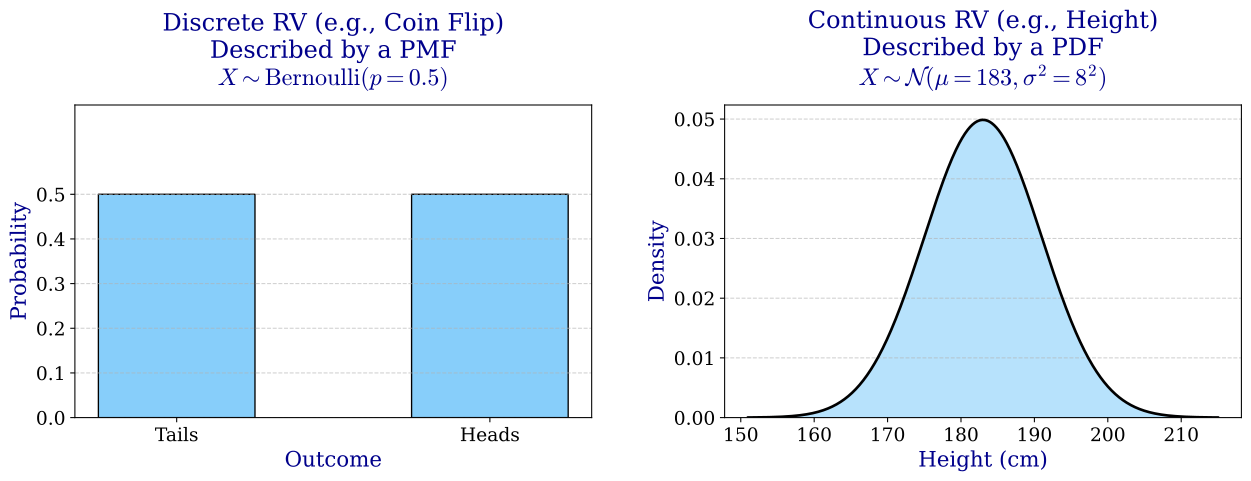
Probability mass function (PMF)
Probability density function (PDF)
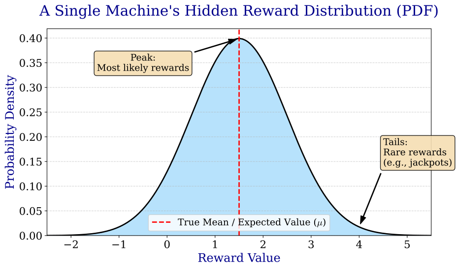
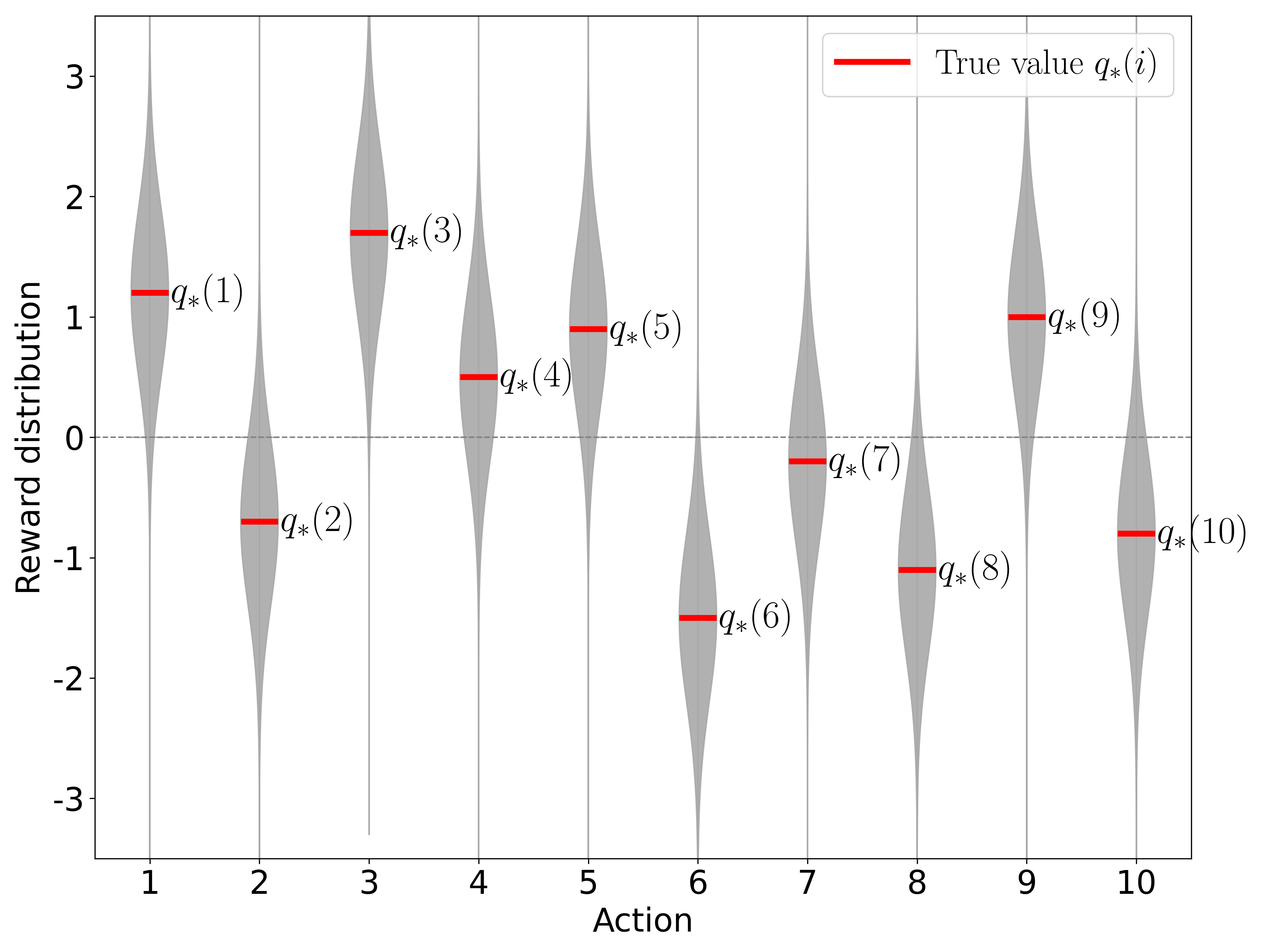
Every machine has a hidden “personality” (Its PDF)
1
Distribution on rewards
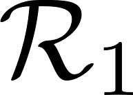
•Represents the true, hidden probability of all possible rewards for a single action.
•The area under a section of the curve gives the probability of a reward falling within that range.
What do we know about these slot machines?
1
Consider the 1st slot machine.
You pull its arm 5 times and observe
the following payouts (rewards ).
= 2
= 1
= -1
= 3
= 0
Why are we receiving
different rewards if the
machine is the same?
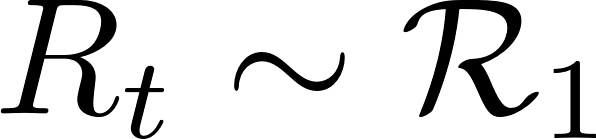
Rewards are sampled
from a distribution!
Reward distribution - Machine 1
What does sampling from a distribution mean? [Review]
Sampling from a probability distribution
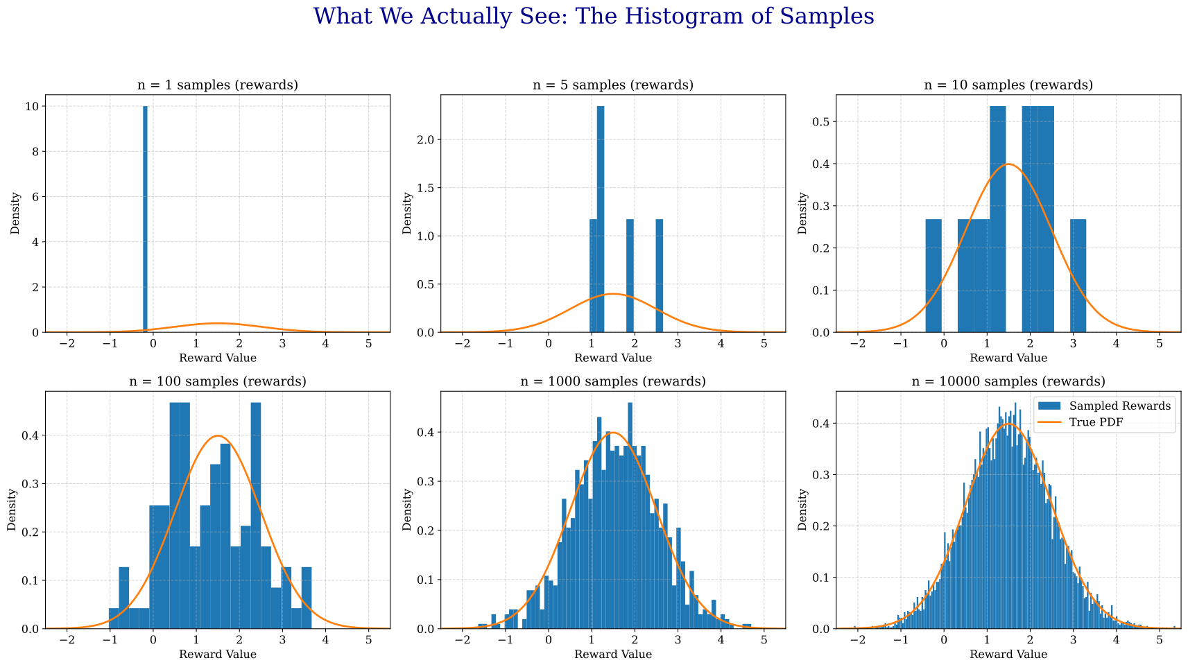
•Sampling from a probability distribution = generate an individual/a data point according to that distribution
•As we collect more samples, the shape of our data converges to the hidden truth.
[Review]
What do we know about these slot machines?
1
Consider the 1st slot machine.
You pull its arm 5 times and observe
the following payouts (rewards ).
= 2
= 1
= -1
= 3
= 0
Why are we receiving
different rewards if the
machine is the same?
What value would you guess for ?
Rewards are sampled
from a distribution!
Reward distribution - Machine 1
The sample mean approximates the true mean.
What is Expected value? [Review]



Expected Value
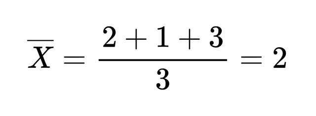
We throw a fair dice and observe 2, 1, 3.
Is this a good summary statistic of the dice?
[Review]
Rolling a Dice
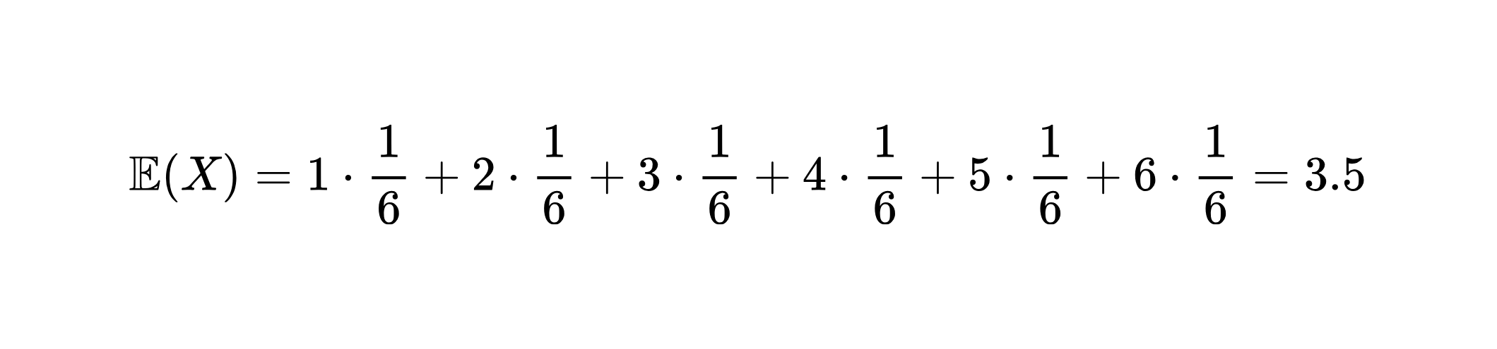
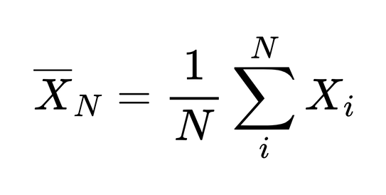
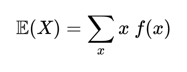
The expected value of an RV is a constant:
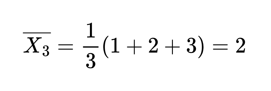
The sample mean depends on the data:
[Review]
Expected Value
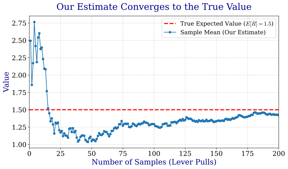
The sample mean
is very different from the expected value
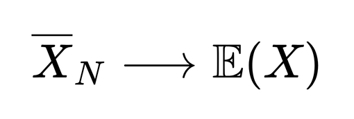
Only in the long run,
[Review]
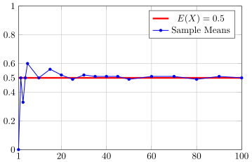
Throwing a Coin
Number of trials
Value
[Review]
Action value estimates
Action 1
Action 2
Action 3
Action 4
Estimated value of action at time step
Which machine would you
decide to choose next?
Why?
Highest estimate
Highest uncertainty
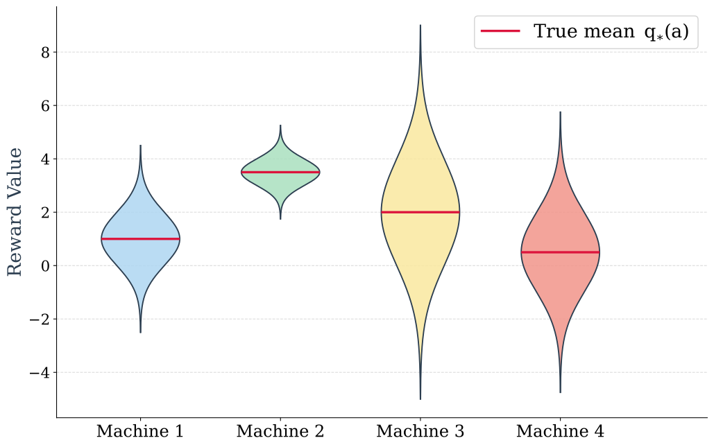
Reward Distributions – 4 Bandits (slot-machines)
Which machine would you
decide to choose next?
Why?
Highest true mean!
Expected reward of action a

Action at time t
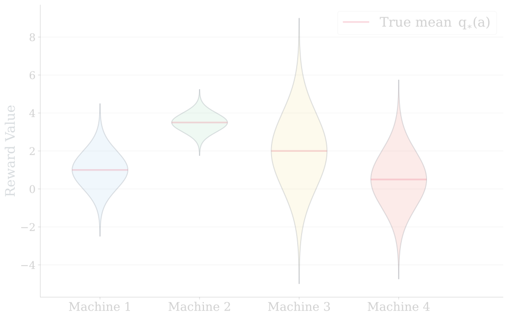
Reward Distributions – 4 Bandits (slot-machines)
Which machine would you
decide to choose next?
Why?
Highest true mean!
Problem:
We do not know the reward distributions a priori!
Expected reward of action a
Action at time t
Formalizing the Multi-Armed Bandit problem
➢Multi-armed bandit: Set of distributions
Set of actions
Distribution on rewards, given action
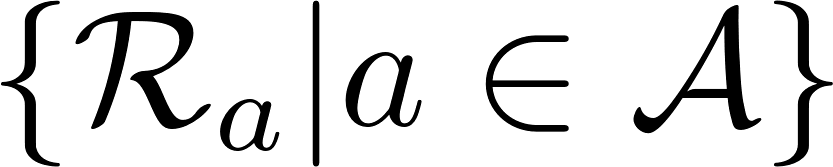
Formalizing the Multi-Armed Bandit problem
➢Multi-armed bandit: Set of distributions
➢At each step , the agent selects an action
Why write instead of ?
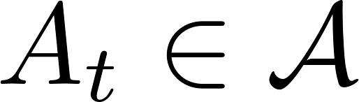
is a random variable
is one fixed action
Formalizing the Multi-Armed Bandit problem
➢Multi-armed bandit: Set of distributions
➢At each step , the agent selects an action
➢The environment generates a reward
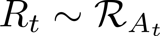
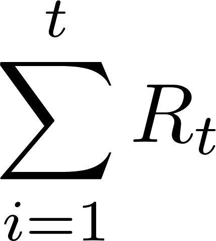
Goal: Maximize cumulative reward
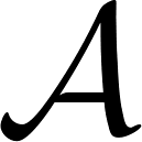
To achieve the goal, we learn a policy : a probability distribution on
Policy
Formally

Why it needs to be between 0 and 1? [Review]
To achieve the goal, we learn a policy : a probability distribution on
Probability Mass Function (PMF)
[Review]
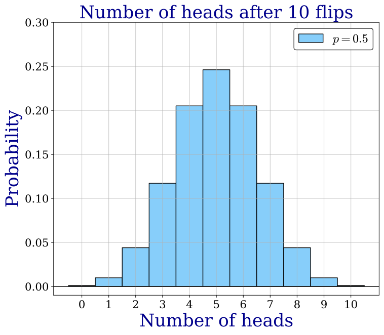
•A function is a valid PMF if it follows two simple rules:
1.Rule 1: All outputs are valid probabilities.
2.Rule 2: The total probability is 1.

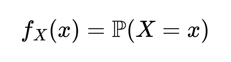
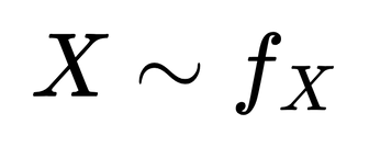
•A PMF describes the probability for each possible outcome of a
discrete random variable.
A Policy is a PMF over actions
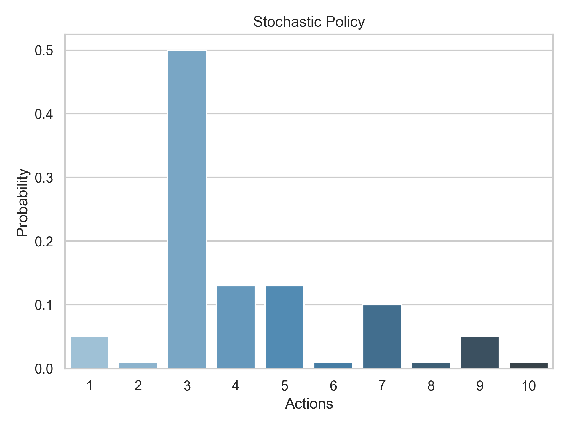
•A policy is simply a PMF where the "outcomes" are
the possible actions the agent can take.
•A policy must follow the same two rules:
Rule 1 Applied to Policies: The probability of selecting any
single action `a` must be between 0 and 1.
Rule 2 Applied to Policies: The probabilities of selecting all
possible actions must sum to 1 (the agent has to choose
something).
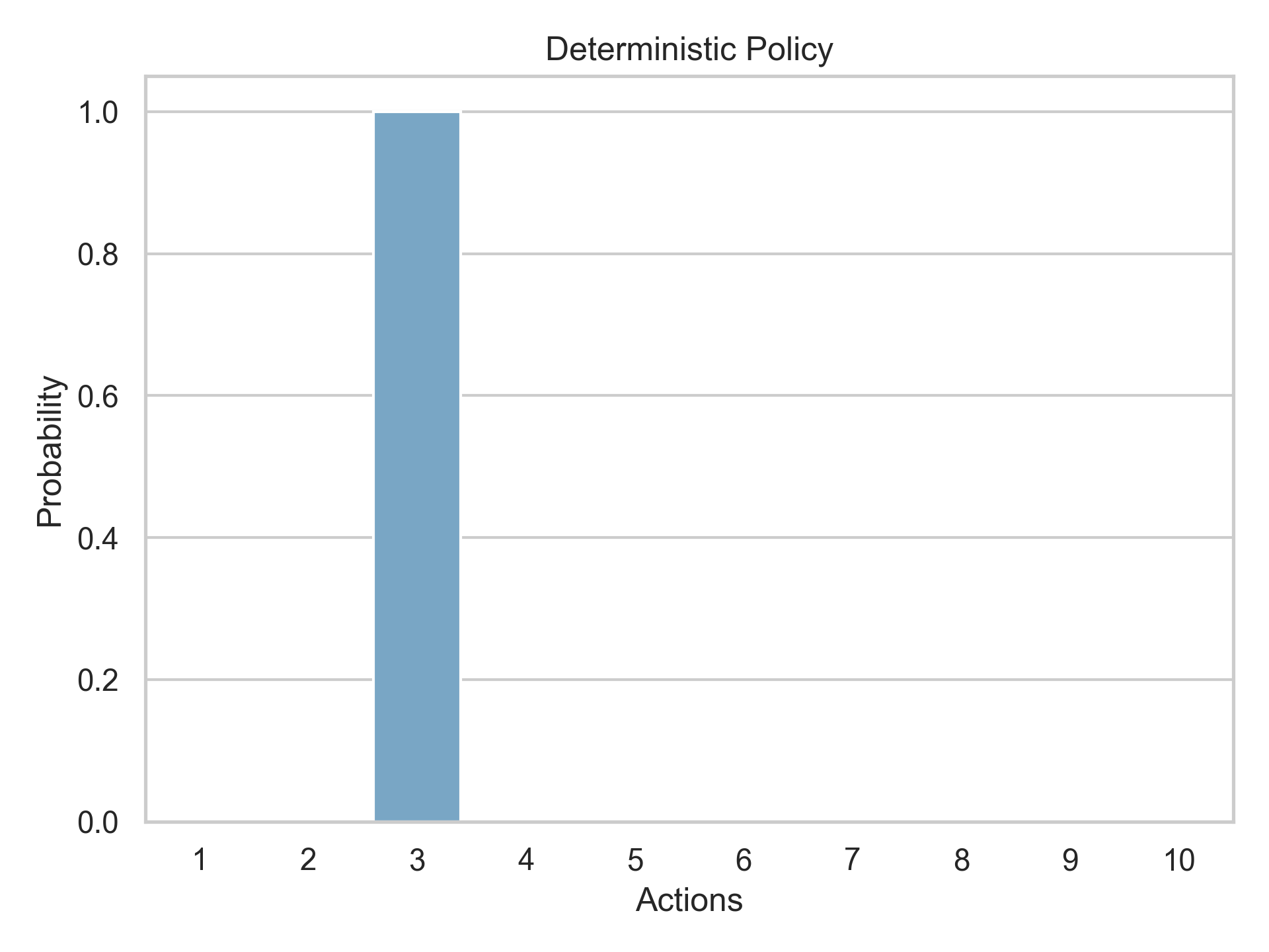
Policy
Action | 1 | 2 | 3 | 4 | 5 | 6 | 7 | 8 | 9 | 10 |
Deterministic | 0 | 0 | 1 | 0 | 0 | 0 | 0 | 0 | 0 | 0 |
Stochastic | 0.05 | 0.01 | 0.50 | 0.13 | 0.13 | 0.01 | 0.10 | 0.01 | 0.05 | 0.01 |
Deterministic X Stochastic policy
To achieve the goal, we learn a policy : a distribution on
Formally

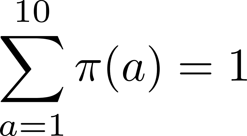
Policy
Action | 1 | 2 | 3 | 4 | 5 | 6 | 7 | 8 | 9 | 10 |
Deterministic | 0 | 0 | 1 | 0 | 0 | 0 | 0 | 0 | 0 | 0 |
Stochastic | 0.05 | 0.01 | 0.50 | 0.13 | 0.13 | 0.01 | 0.10 | 0.01 | 0.05 | 0.01 |
Deterministic X Stochastic policy
How to find the optimal policy?
Action-Value Methods
➢First: Learn the reward distribution, or just its mean (action values)
➢Second: Find a policy based on the action values
■Greedy
■-greedy
■Upper Confidence Bound (UCB)
■Softmax policy
Action-Value function
To achieve the goal, we learn a policy : a distribution on
Action-Value Methods
The action-value function for action is the expected reward
The optimal action is

The Regret of an optimal action is zero.
The Regret of an action is

Sample-Average Method: Direct Average
Time t | Action 1 | Action 2 | Action 3 |
t = 1 | |||
t = 2 | |||
t = 3 | |||
t = 4 | |||
t = 5 | |||
t = 6 |



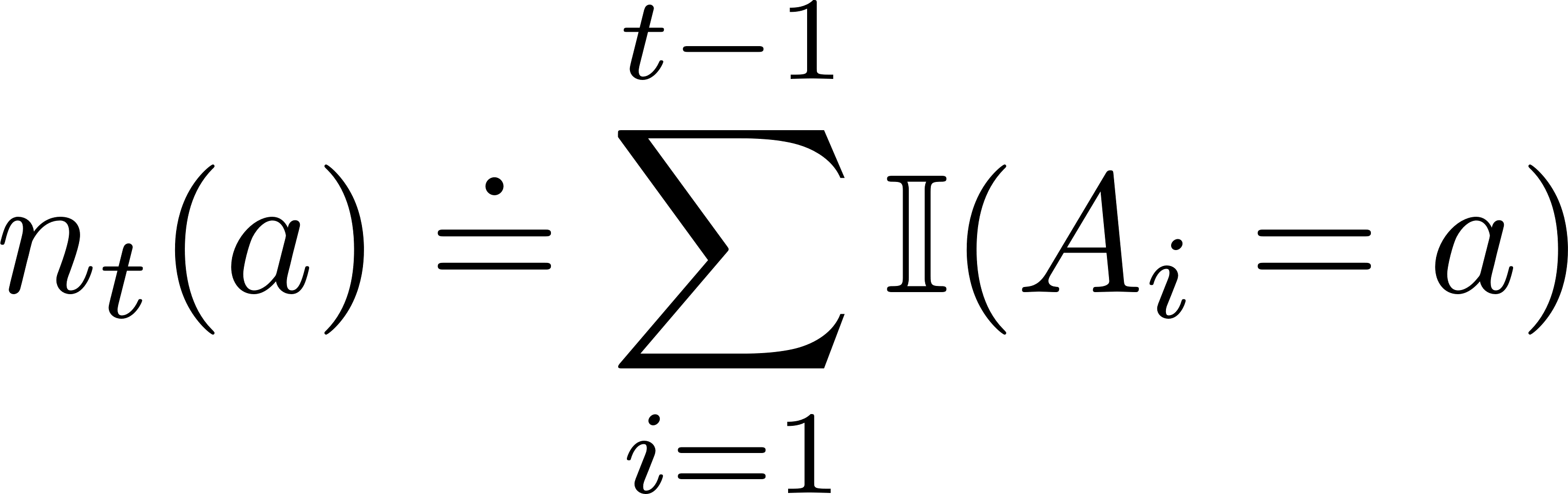
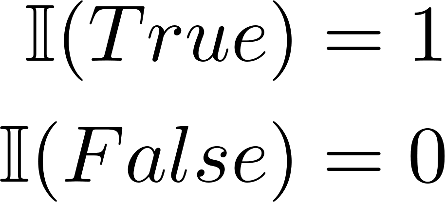
Indicator function:

Sampling Rewards
Sample-Average method: Incremental Implementation
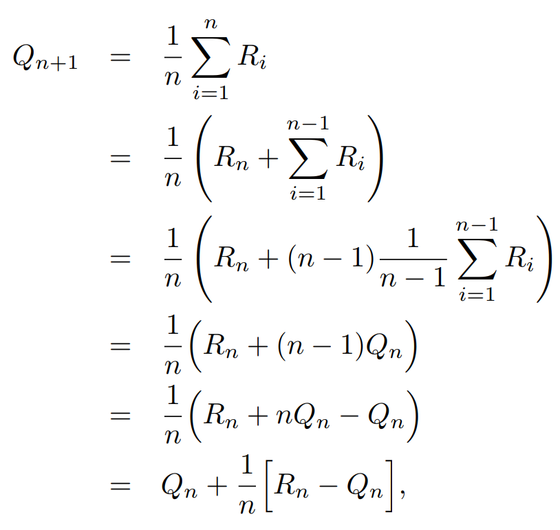
Consider only one action
: reward received after the th selection of this action
: Estimate of its action value after it has been selected times.
Extending to multiple actions






Error in the estimate!
Reduced by taking a step toward the “target”
Sample-Average method: Incremental Implementation
Sample-average method is appropriate for stationary bandit problems
reward probability distribution do not
change over time
Variable StepSize
Stationary bandit problems
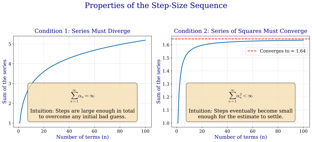
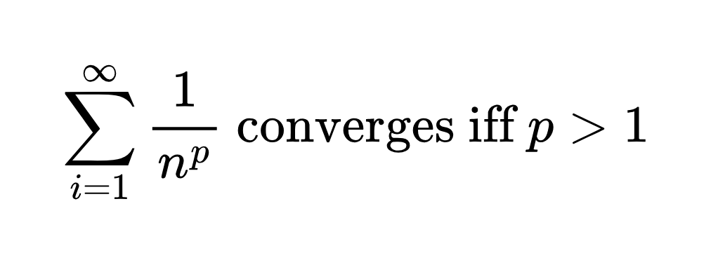
What are the properties of this variable step size? [Review]
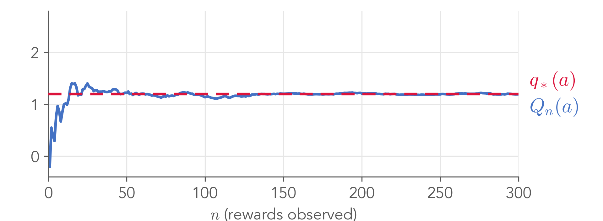
Why the Step-Size Guarantees Learning
[Review]
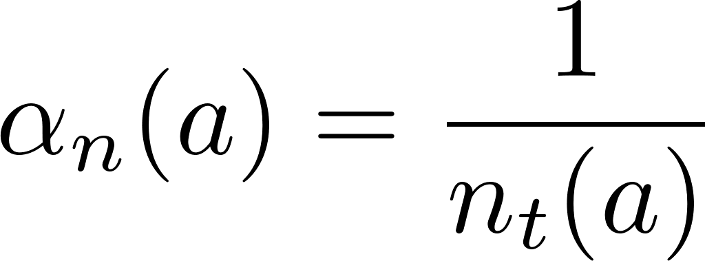
The Step-Size forms a sequence.
A series is the sum of that sequence.
Sample-average method
(more suitable for stationary bandit)
How to compute the action-value function?
Weight-average method
?
Nonstationary
problems
Give more weight to
recent rewards than to
long-past rewards
Use constant StepSize
parameter!

What means ?
Tracking a Nonstationary Problem (Weight-average method)
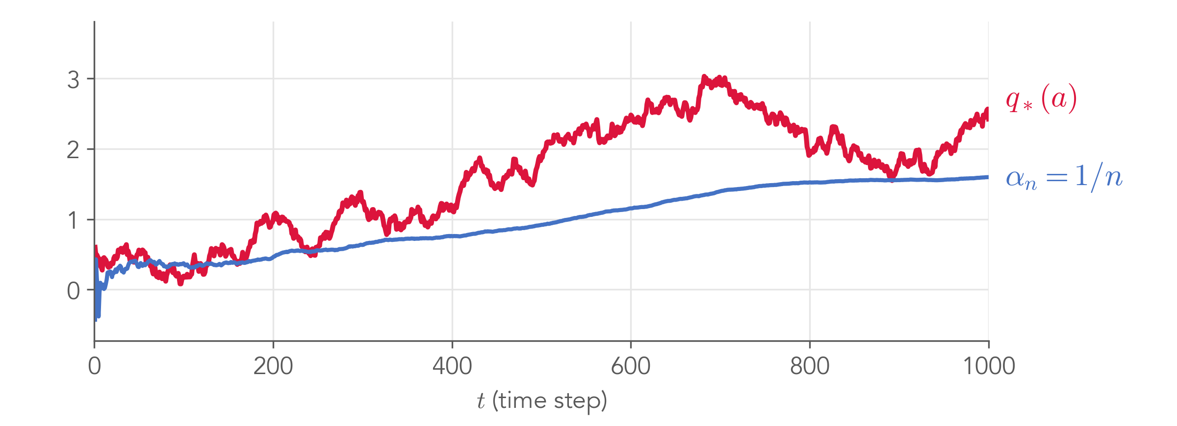
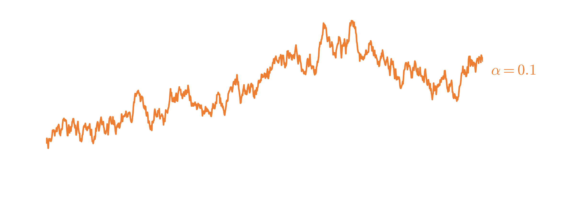
Nonstationary
problems
Give more weight to
recent rewards than to
long-past rewards
Use constant StepSize
parameter!
Tracking a Nonstationary Problem (Weight-average method)
From stochastic
approximation theory
Conditions required to
assure convergence
with probability 1
Does a constant satisfy
these conditions?
Steps are large enough to overcome any
initial conditions or random fluctuations

Steps become small enough to
assure convergence

Nonstationary
problems
Give more weight to
recent rewards than to
long-past rewards
Use constant StepSize
parameter!
Tracking a Nonstationary Problem (Weight-average method)
Which satisfies
these conditions?
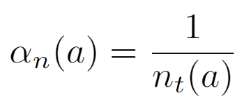
Sample-average method

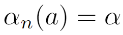
Weight-average method

Estimates never completely converge but
continue to vary in response to the most
recently received rewards.
Desirable in a
nonstationary
environment!
Usually the case in
Reinforcement
Learning problems.
Nonstationary
problems
Give more weight to
recent rewards than to
long-past rewards
Use constant StepSize
parameter!
Tracking a Nonstationary Problem (Weight-average method)

More details in
book’s page 32.
Nonstationary
problems
Give more weight to
recent rewards than to
long-past rewards
Use constant StepSize
parameter!
Tracking a Nonstationary Problem (Weight-average method)
Initial estimate
Past rewards
weighted average
Sample-average method
(more suitable for stationary bandit)
How to compute the action-value function?
Weight-average method
(suitable for stationary and nonstationary bandit)
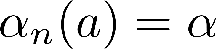

Algorithms: Action-value methods
Greedy
UCB
Softmax
-greedy
Action-value update rule
Policies
Greedy
Select the action with the highest estimated value
(It always exploits)
Problems?
Suppose that our current estimates are
represented by
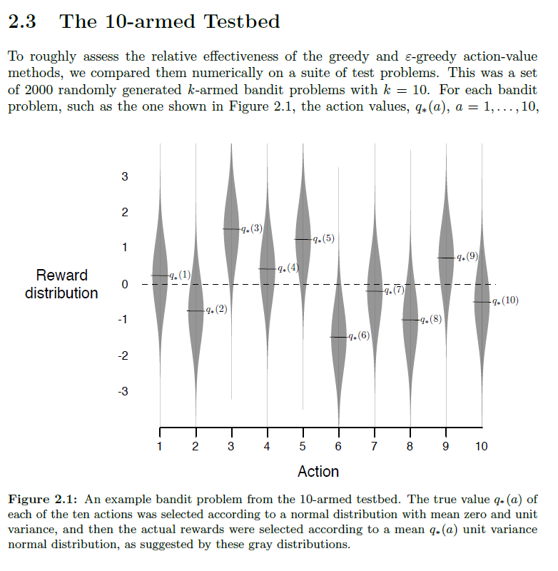
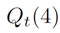
We would keep selecting action 4 for how long?
In which suboptimal will we get stuck?
Does this induce a
deterministic or
stochastic policy?

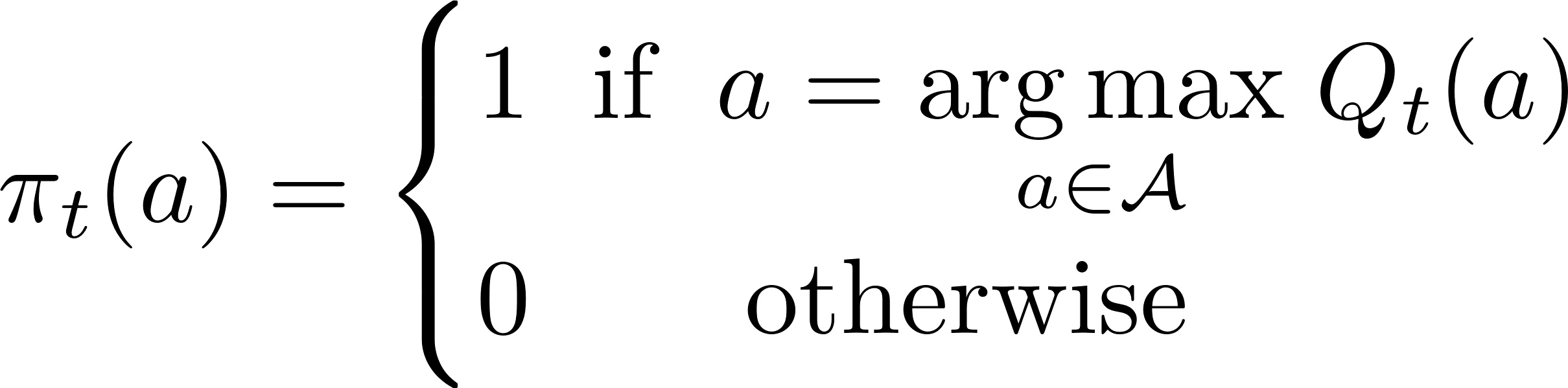
Greedy
Select the action with the highest estimated value
Problems?
Suppose that our current estimates are
represented by
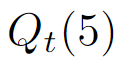
It’s an estimated value! It can be wrong.
We will get stuck in a suboptimal forever!
Greedy
Select the action with the highest estimated value
Problems?
It’s an estimated value! It can be wrong.
We will get stuck in a suboptimal forever!
Suppose that our current estimates are
represented by
Suboptimal: Action 5
Optimal action: Action 3
Greedy
Select the action with the highest estimated value
Problems?
It’s an estimated value! It can be wrong.
We will get stuck in a suboptimal forever!
Suppose that our current estimates are
represented by
We need to find a way to keep updating the
action value estimates of the other actions!
Algorithms: Action-value methods
Greedy
UCB
Softmax
?
?
?
-greedy
-greedy
Small number
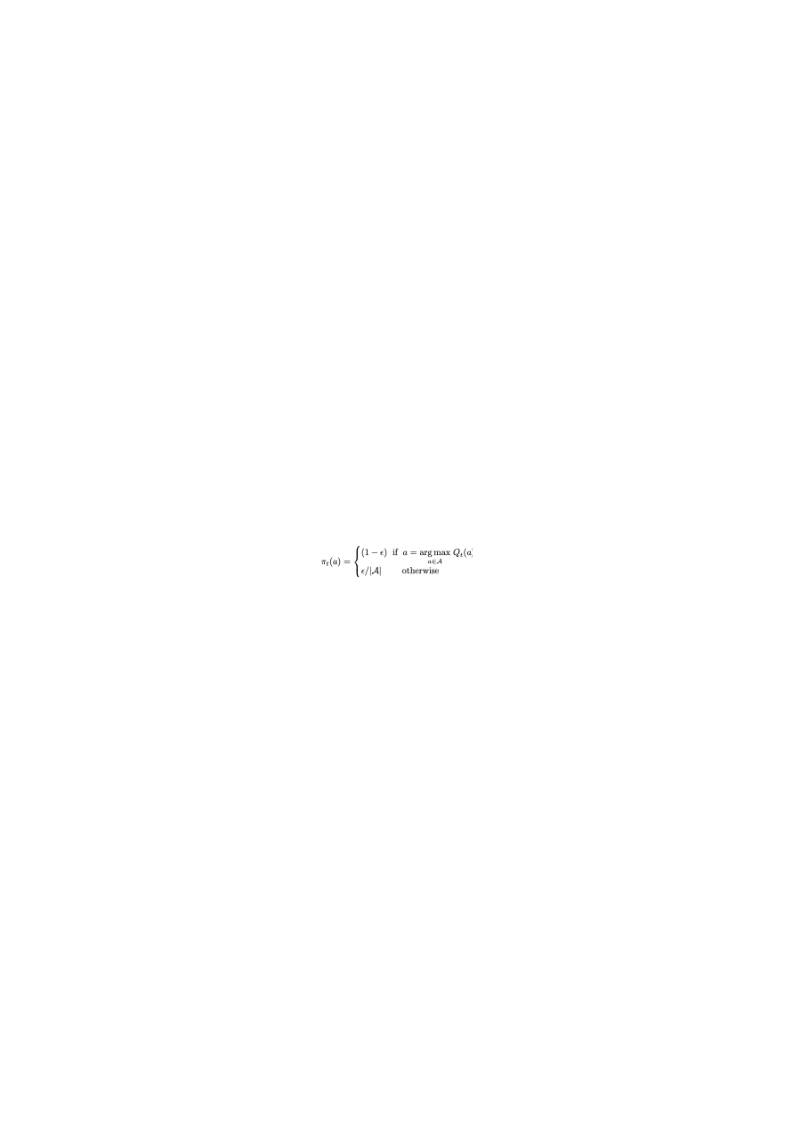
Is this expression representing
the above sentences?
➢Behave greedily with probability
➢Take a random action with probability
(It keeps exploring!)

-greedy
Small number
➢Behave greedily with probability
➢Take a random action with probability
(It keeps exploring!)
Example:



Actions | 1 | 2 | 3 | 4 | |
Action-value estimates | 3 | 1 | 4 | -2 | |
Probabilities | Exploit () | ||||
Explore (Uniformly random) | |||||
𝜖-greedy policy | |||||


-greedy
Small number
➢Behave greedily with probability
➢Take a random action with probability
(It keeps exploring!)
Example:
Actions | 1 | 2 | 3 | 4 | |
Action-value estimates | 3 | 1 | 4 | -2 | |
Probabilities | Exploit () | 0 | 0 | 0.6 | 0 |
Explore (Uniformly random) | 0.1 | 0.1 | 0.1 | 0.1 | |
𝜖-greedy policy | |||||
-greedy
Small number
➢Behave greedily with probability
➢Take a random action with probability
(It keeps exploring!)
Example:
Actions | 1 | 2 | 3 | 4 | |
Action-value estimates | 3 | 1 | 4 | -2 | |
Probabilities | Exploit () | 0 | 0 | 0.6 | 0 |
Explore (Uniformly random) | 0.1 | 0.1 | 0.1 | 0.1 | |
𝜖-greedy policy | 0.1 | 0.1 | 0.7 | 0.1 | |


-greedy
Small number
Is this expression representing
the above sentences?
➢Behave greedily with probability
➢Take a random action with probability
(It keeps exploring!)
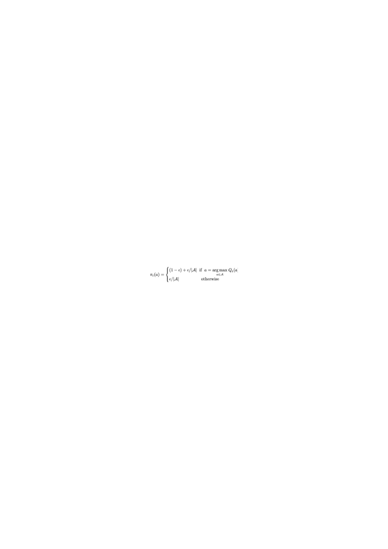
-greedy policy
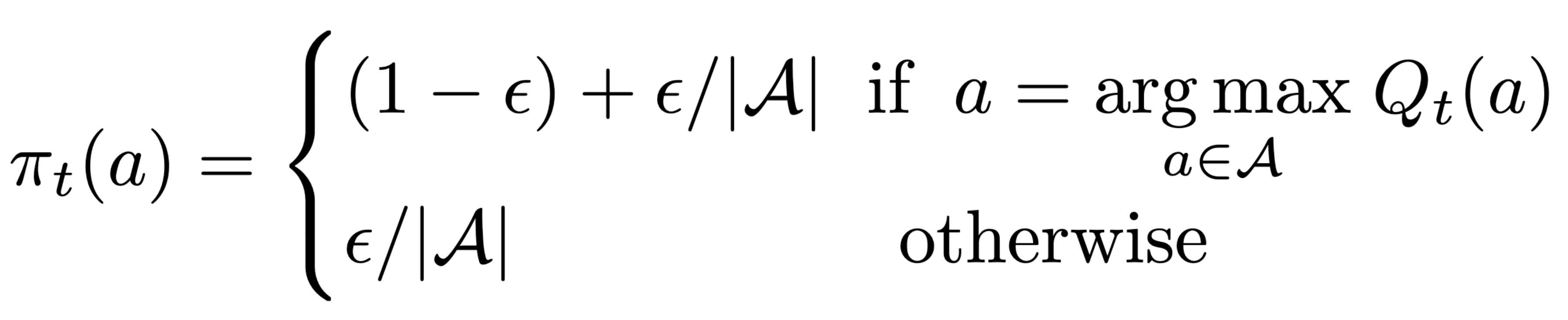
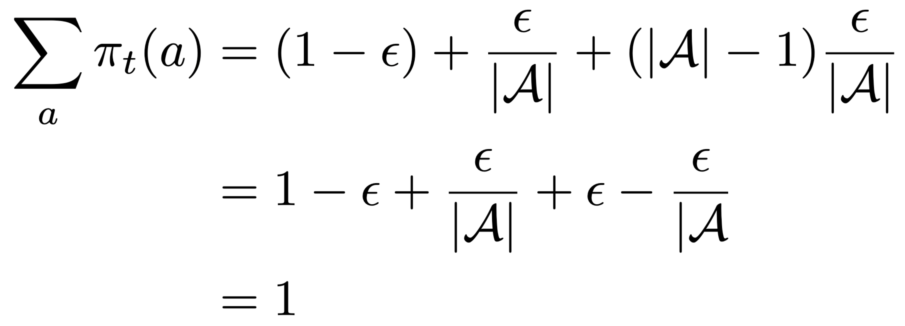
Rule 1: All outputs are valid probabilities.
Rule 2: The total probability is 1.
?
?
Is the -greedy policy a pmf?
Greedy x e-greedy
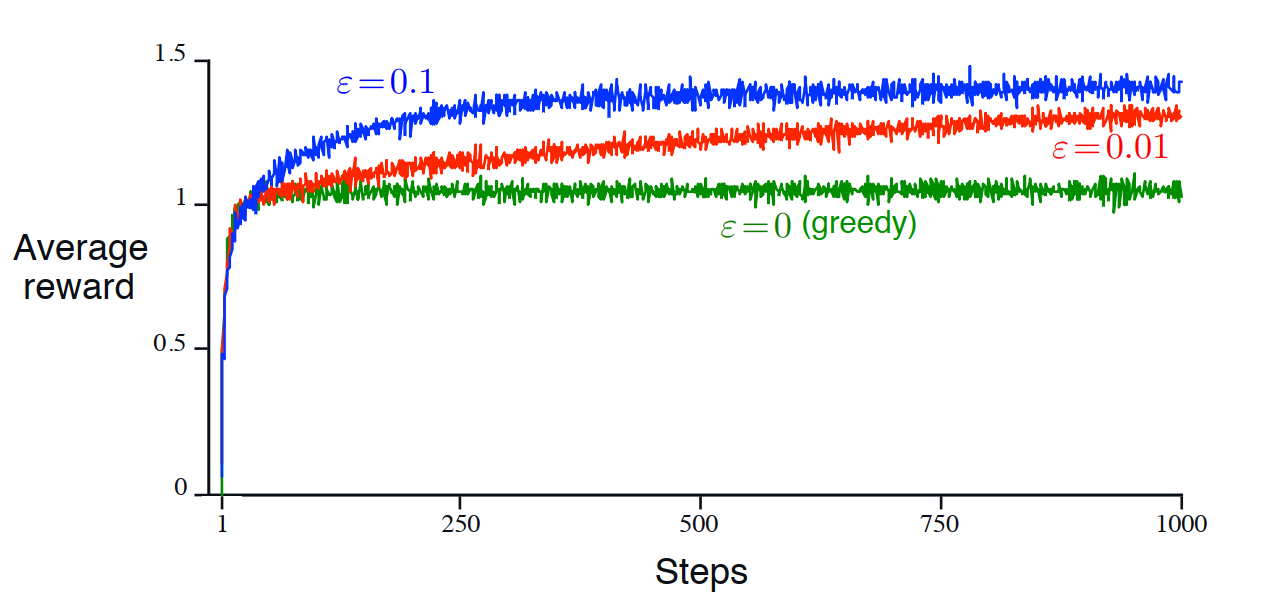
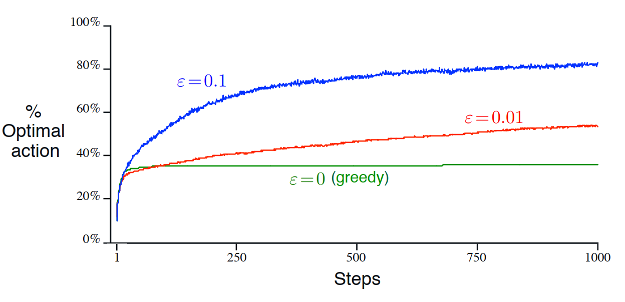
Average performance of -greedy action-
value methods on the 10-armed testbed.
A simple bandit algorithm (e-greedy)
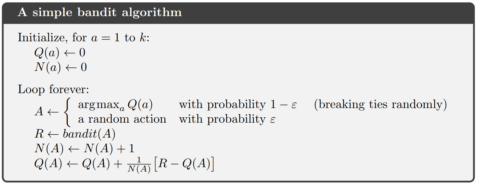
A simple bandit algorithm (e-greedy)
Is this a good initialization? Is there a way that improves exploration?
Using Optimistic Initial Values
Greedy algorithm
Initializing action-values as 0
Initializing action-values optimistically
What is the maximum value that can be
obtained in a normal distribution?
Using Optimistic Initial Values
Greedy algorithm
Suppose action 9 is selected.
Initializing action-values as 0
Initializing action-values optimistically
Using Optimistic Initial Values
Greedy algorithm
Greedy will keep selecting action 9
Greedy will select all other actions several
times before the value estimates converge!
Initializing action-values as 0
Initializing action-values optimistically
Using Optimistic Initial Values
Greedy algorithm
Greedy will keep selecting action 9
Initializing action-values as 0
Initializing action-values optimistically
Greedy will select all other actions several
times before the value estimates converge!
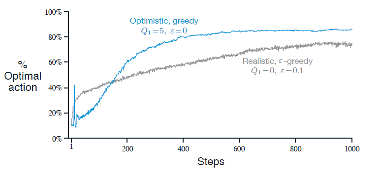
Effect of using Optimistic Initial Values

Algorithms: Action-value methods
Greedy
UCB
Softmax
?
?
-greedy
Optimism in the Face of Uncertainty
Up to now, we are considering only the action-value estimates to derive a policy.
3
2
1
0
-1
-2
-3
123
Action
Estimated
action values
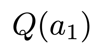
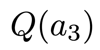
What if we could consider the
uncertainty of our estimates?
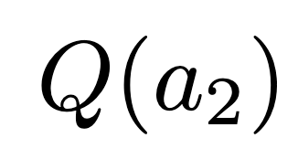
Optimism in the Face of Uncertainty
Up to now, we are considering only the action-value estimates to derive a policy.
3
2
1
0
-1
-2
-3
123
Action
Estimated
action values
What if we could consider the
uncertainty of our estimates?
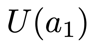
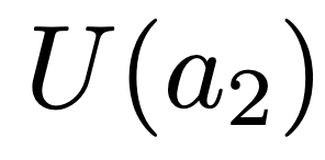
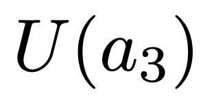
Uncertainty in the
estimation of
Optimism in the Face of Uncertainty
Up to now, we are considering only the action value estimates to derive a policy.
3
2
1
0
-1
-2
-3
123
Action
Estimated
action values
What if we could consider the
uncertainty of our estimates?
Uncertainty in the
estimation of
Acting greedy with respect to the
action-value results in action 1.
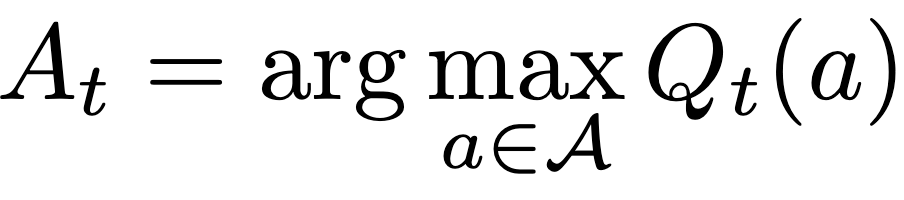
Acting greedy with respect to the
action-value + uncertainty results
in action 2!

Optimism in the Face of Uncertainty
Up to now, we are considering only the action value estimates to derive a policy.
3
2
1
0
-1
-2
-3
123
Action
Estimated
action values
Acting greedy with respect to the
action-value + uncertainty results
in action 2!
After selecting action 2, we got new
information and reduce our uncertainty
and update the action-value estimate.
How can we compute this uncertainty?
Which property should it have?
Upper Confidence Bound (UCB)
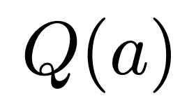
We want to estimate an upper confidence
bound for every action value

3
2
1
0
-1
-2
-3
a
Action
Estimated
action values
Estimate
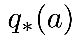
True Value
Upper confidence
bound
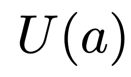
Uncertainty
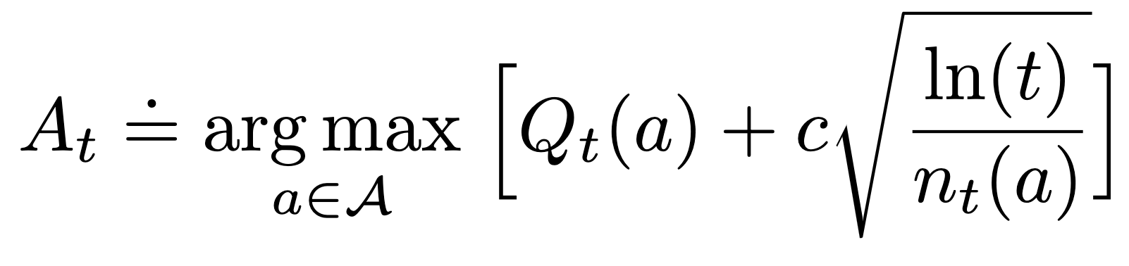
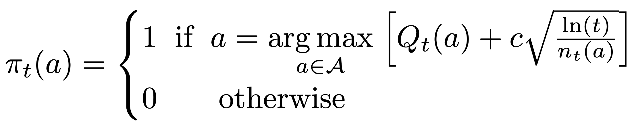
Upper Confidence Bound (UCB)
Increases with time,
increasing uncertainty
scales the
uncertainty! Regulates the
amount of exploration.
Increases when action
a is selected,
decreasing uncertainty.

Upper Confidence Bound (UCB)
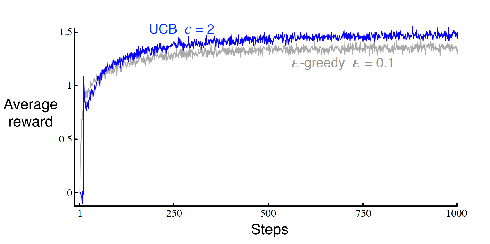
UCB generally performs better than -greedy on the multi-armed bandit problem.
Algorithms: Action-value methods
Greedy
UCB
Softmax
?
-greedy
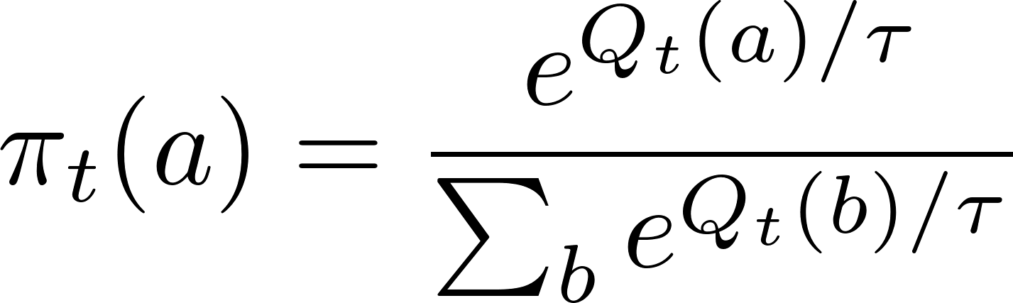
Softmax Action Selection policy
It is possible to produce a stochastic policy from the action-value estimates.
Taking the greedy action is not the only possibility!
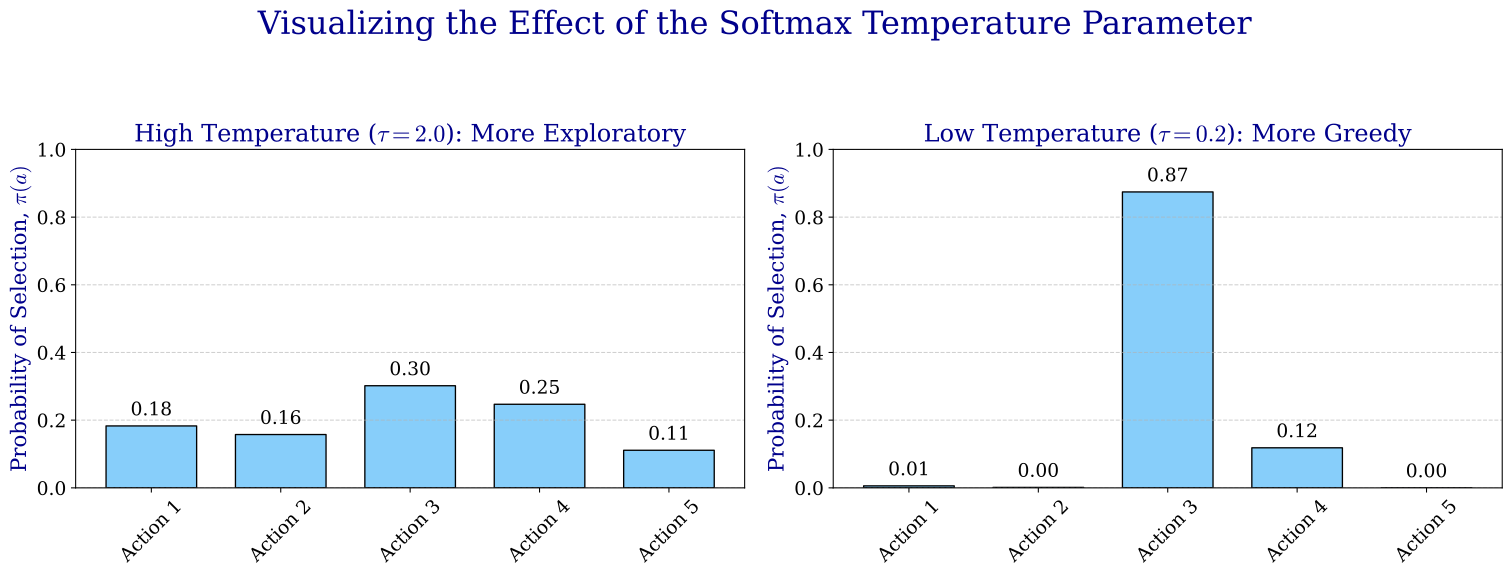
Temperature.
High values => actions (nearly) equiprobable.
Low values => the value estimator has more weight.
Softmax Action Selection policy
Is the softmax action selection policy a pmf?
Rule 1: All outputs are valid probabilities.
Rule 2: The total probability is 1.
?
?
Try to do it at home!
Softmax Action Selection policy
As the estimates converge, what does the softmax policy become?
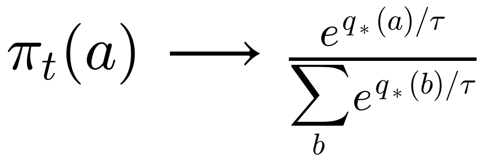
a fixed stochastic policy
τ | P(best action) | expected reward |
1 | 0.32 | 0.81 |
0.25 | 0.74 | 1.45 |
0.1 | 0.89 | 1.53 |
10-armed testbed, true values drawn from N(0, 1); optimal expected reward 1.54
With a fixed , the policy converges to softmax(): it learns a policy, but not the optimal
one.
Algorithms: Action-value methods
Greedy
-greedy
UCB
Softmax
Policy gradient methods
Goal: Maximize cumulative reward
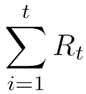
To achieve the goal, we learn a policy : a distribution on
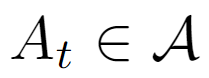
Multi-armed bandit problem
Instead of learning first and then deriving , why not learn directly?
Policy gradient methods
Idea: update policy parameters such that expected value increases
Use a policy parameterized by :
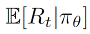
Use gradient ascent to update


Policy gradient methods
Idea: update policy parameters such that expected value increases
Use a policy parameterized by :
Use gradient ascent to update
Step-size between 0 and 1
“How fast is updated”
Policy gradient methods
Idea: update policy parameters such that expected value increases
Use a policy parameterized by :
Use gradient ascent to update
How to compute this gradient?
Policy gradient methods


Definition of conditional
expectation on our policy.

Policy gradient methods
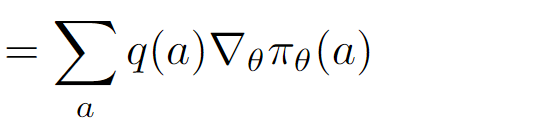
Policy gradient methods
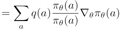
Policy gradient methods
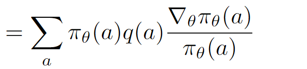
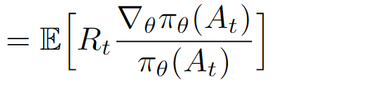
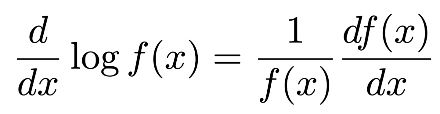
Policy gradient methods

Policy gradient methods
Gradient ascent

From previous derivation.
We can sample this and use stochastic gradient ascent on the (true) value of the policy.

We can use sampled rewards! It does not need value estimates.
Action preferences
Consider a Softmax policy based on action preferences
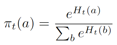
The preferences are learnable policy parameters.
Goal: learn by optimizing the preferences with stochastic gradient ascent.
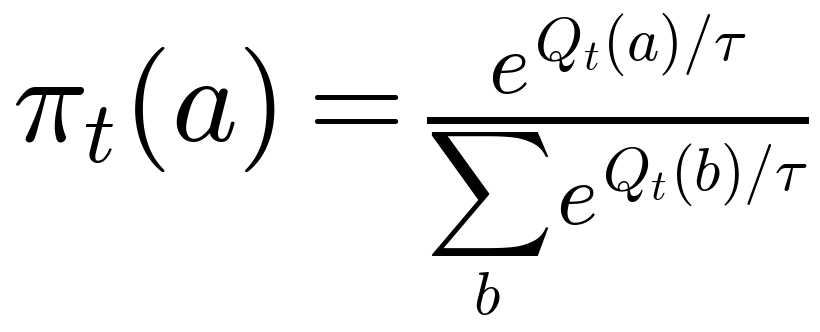
action values
action preferences
→ , so the action-value policy converges to softmax(). has no fixed target.
Action Preferences

Softmax policy
Stochastic Gradient ascent
Derivation of the
update rule


Action Preferences
➢Preferences for actions with higher rewards increase more (or decrease less), making them more
likely to be selected again.
Update Rule
Stochastic Gradient ascent
Softmax policy
Action Preferences with baseline
Update Rule
To mitigate this, we can keep tracking of the average of the
rewards up to but not including time (with ), and
consider it as a baseline.
Recall that the sampled
reward at each time-step
has high variance.
1) = 2
2) = 1
3) = -1
4) = 3
5) = 0
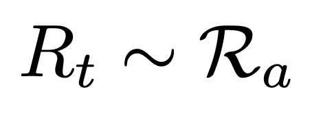

Update Rule with baseline
More details on page 38 of the book.
Action Preferences
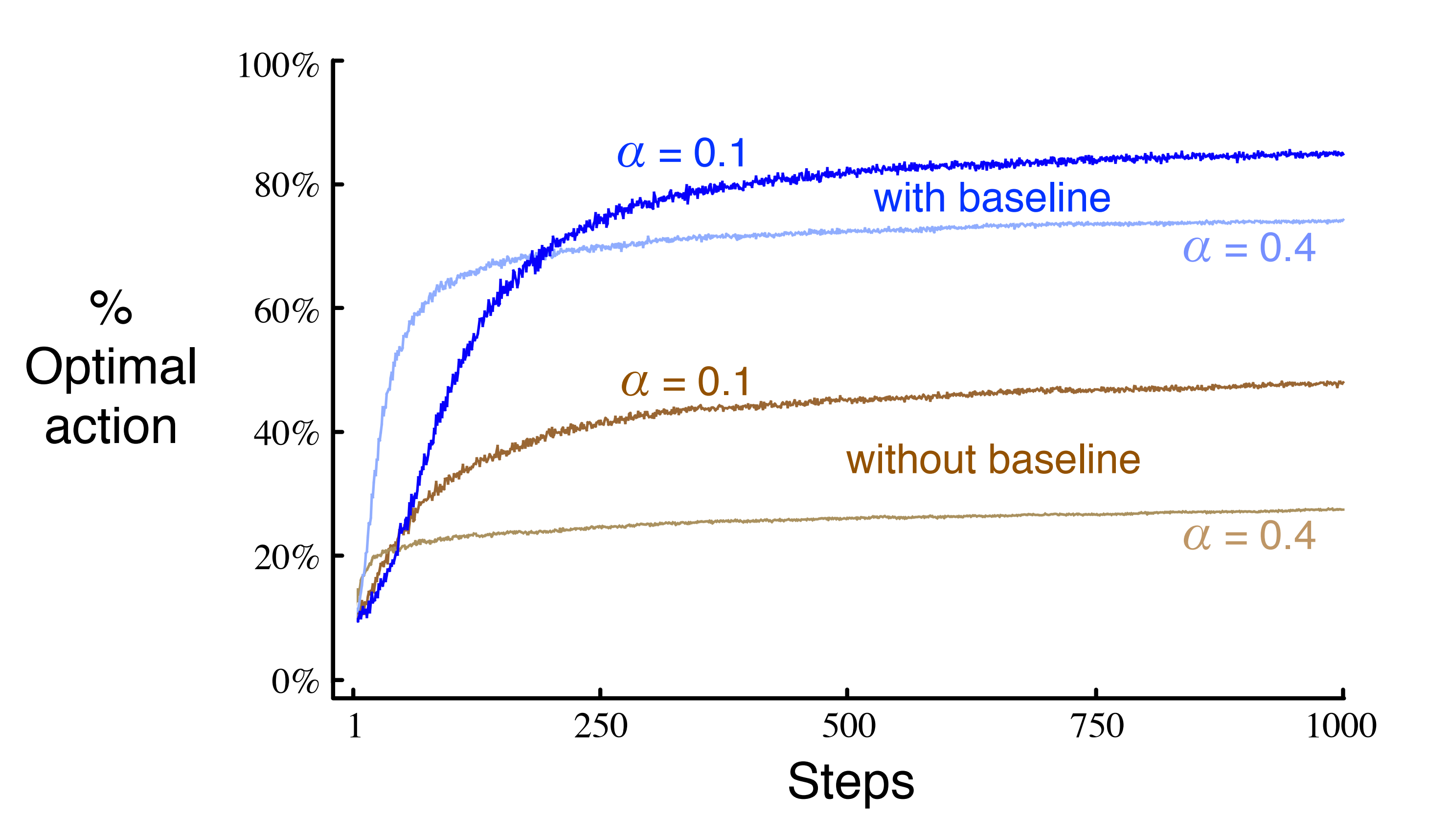
Average performance of the gradient bandit algorithm with and without a reward
baseline on the 10-armed bandit testbed.
Action Values vs Action Preferences
10-armed testbed, true values drawn from N(0, 1); average of 2,000 runs
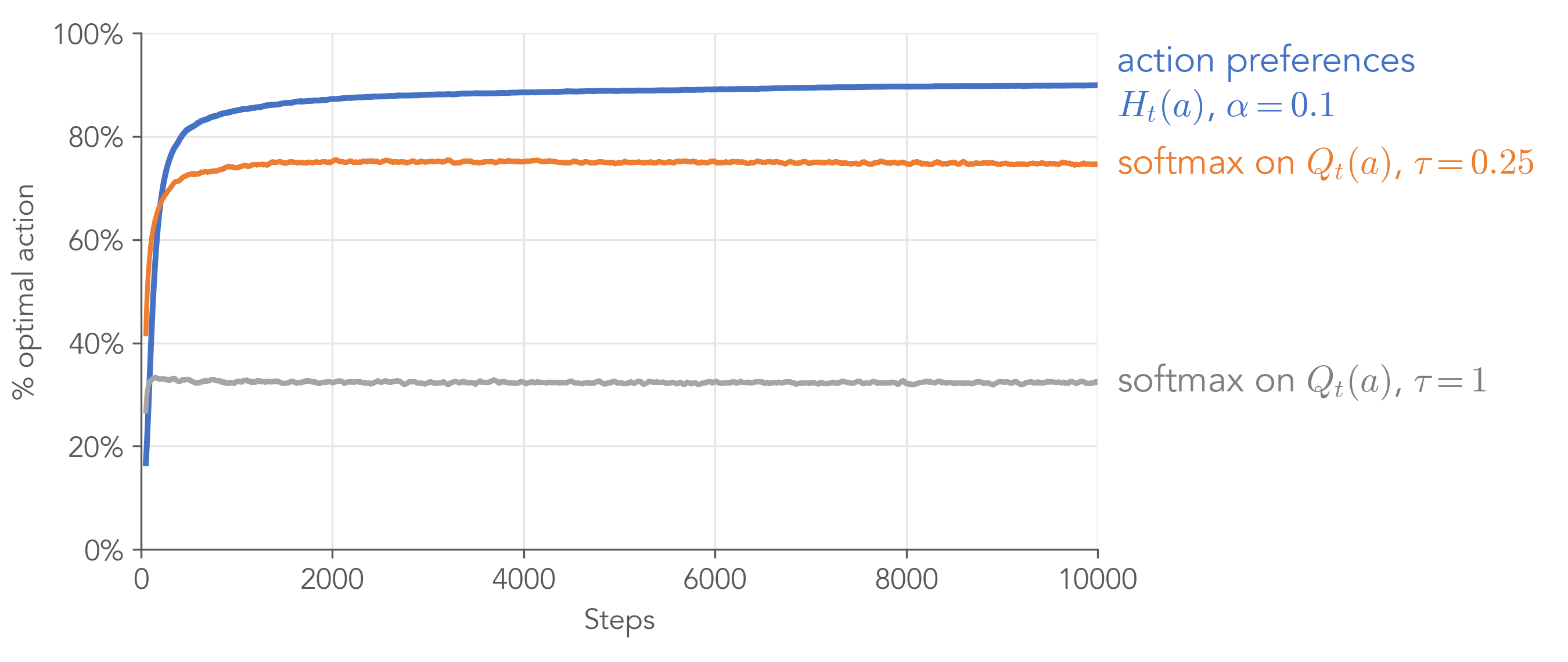
Softmax on : converges to softmax(), a fixed stochastic policy.
Action preferences : no fixed target, so the policy becomes nearly deterministic: on the best
action in about 9 of 10 runs, otherwise mostly on the second best.
Algorithms: Policy gradient based
Action
Preferences
Policy
Action Preference update rule
Algorithm
Action Preference update rule with baseline
Summary
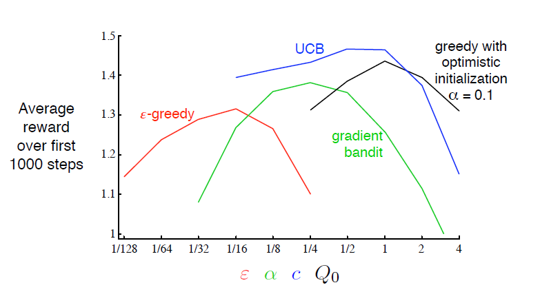
Parameter study of various bandit algorithms. Each point is the average reward obtained
over 1000 steps with a particular algorithm at a particular setting of its parameter.
See book’s page 42 for details.