
Reinforcement Learning · Lecture 2

The RL problem and Finite MDP
Rafael Fernandes Cunha

rafaelcunha2013.github.io

Today’s topics

1.Recap on exploration methods

2.The Reinforcement Learning (RL) framework

3.The Markov Decision Process (MDP)

4.Returns

5.Policies

6.Value functions

7.Bellman equations

2

1.Describe the RL framework.

2.Create an environment as an MDP.

3.Describe the goal of the RL agent.

4.Describe why value functions can be used to
evaluate a policy.

5.Explain the recursive nature of Bellman equations.

Learning outcomes

Recap on Exploration Methods

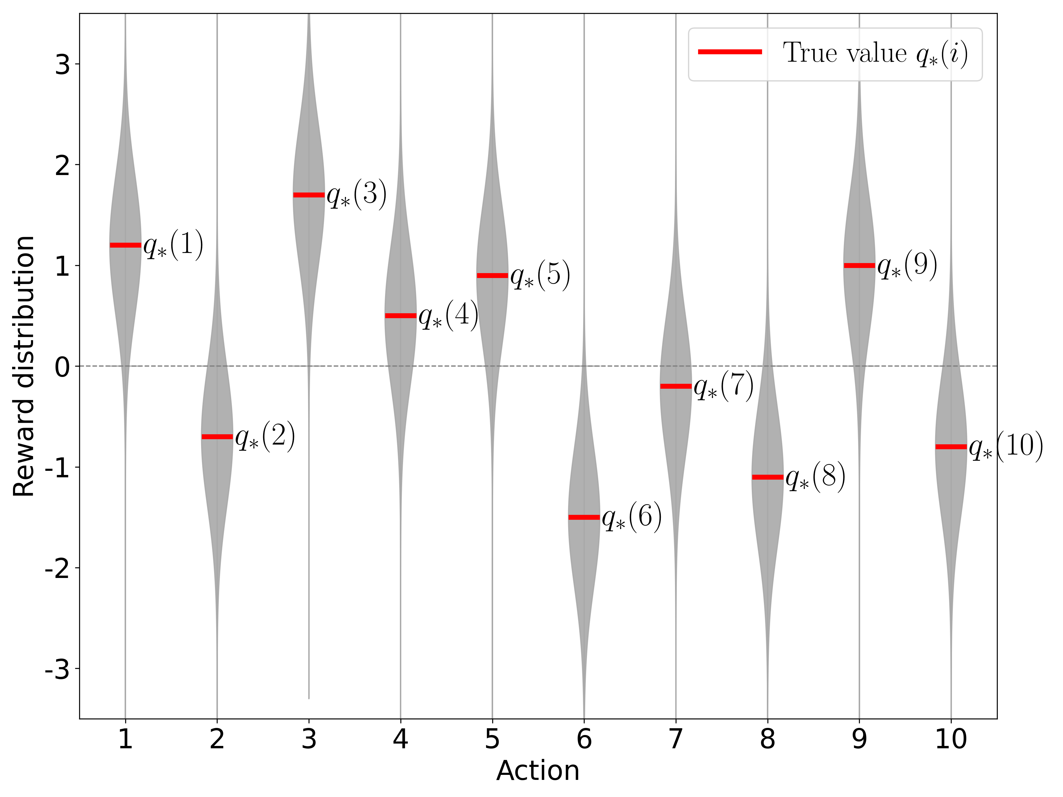
Formalizing the Multi-Armed Bandit problem

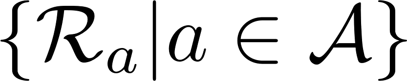
➢Multi-armed bandit: Set of distributions

​

​

​

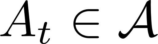
➢At each step , the agent selects an action

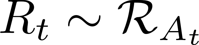
➢The environment generates a reward
\begin{align*}
\{\mathcal{R}_a | a \in \mathcal{A}\}
\end{align*}
\begin{align*}
A_t \in \mathcal{A}
\end{align*}
\begin{align*}
 R_t \sim  \mathcal{R}_{A_t}
\end{align*}

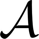
To achieve the goal, we learn a policy : a distribution on
\begin{align*}
\mathcal{A}
\end{align*}

Goal: Maximize cumulative reward

\begin{align*}
\sum_{i=1}^t R_i 
\end{align*}

Update rule

NewEstimate

OldEstimate

StepSize

InformativeValue

Target – OldEstimate

Error

Gradient

Learning Rate

Fixed or variable

Vector

Table

Weights of a NN

Action-value update rule

Sample-average method

Weight-average method

\begin{align*}
Q_{n+1}(a) = Q_n(a) + \alpha_n(a) \Big[ R_n - Q_n(a) \Big]
\end{align*}

From stochastic
approximation theory

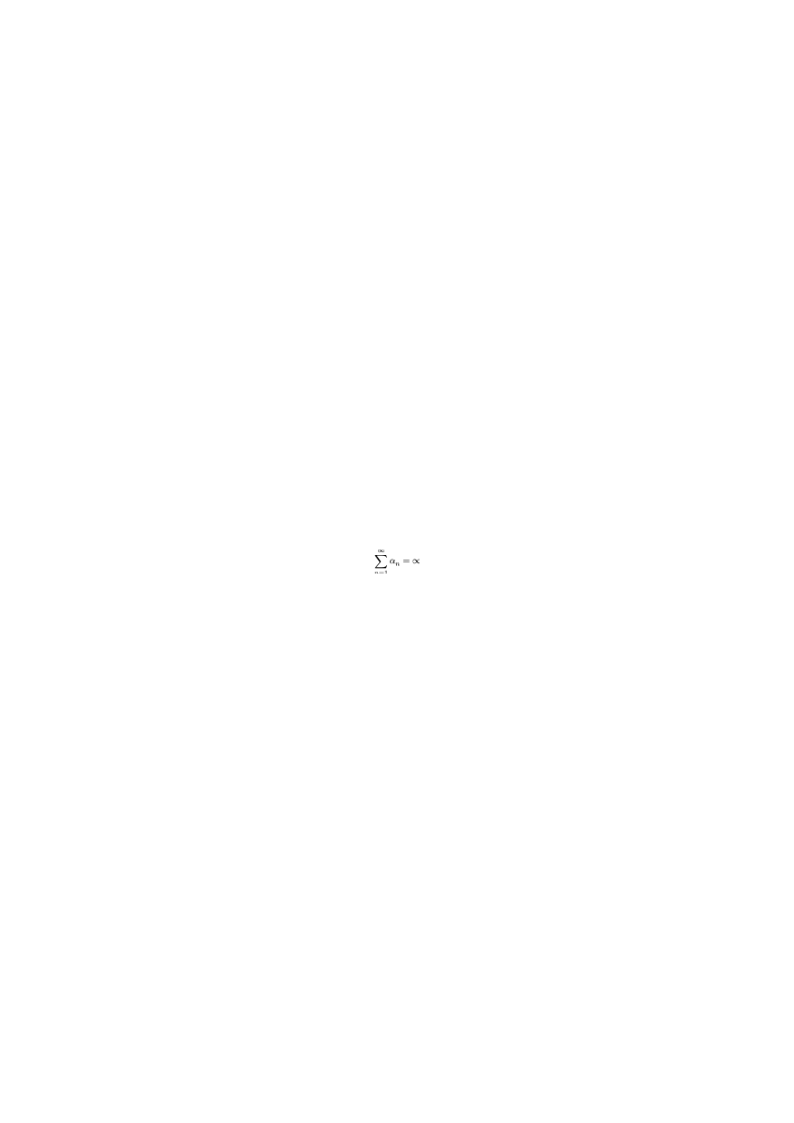
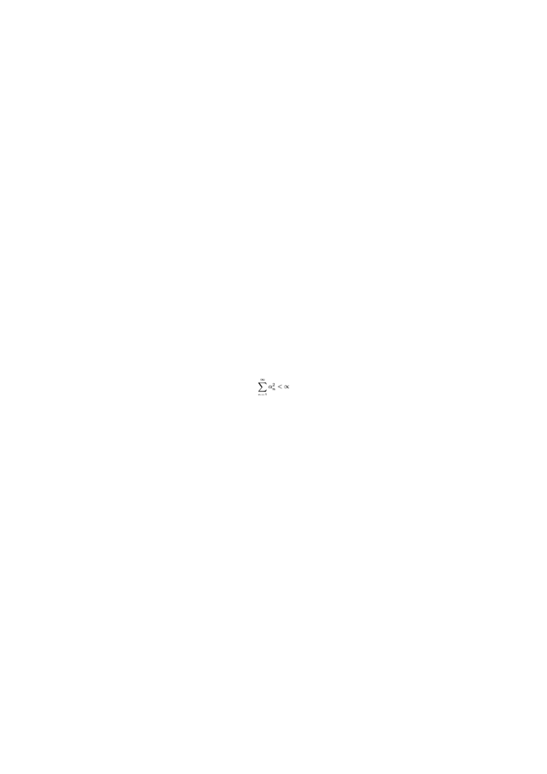
Conditions required to
assure convergence
with probability 1

Steps are large enough to overcome any
initial conditions or random fluctuations
\begin{align*}
    \sum_{n=1}^{\infty} \alpha_n = \infty
\end{align*}

Steps become small enough to
assure convergence
\begin{align*}
    \sum_{n=1}^{\infty} \alpha_n^2 < \infty
\end{align*}

Sequences that meet these conditions are usually:

​

➢Slow to converge.

➢Need considerable tunning for a satisfactory convergence rate.

➢Often used in theoretical work.

➢Not very used in applications and empirical research.

\begin{align*}
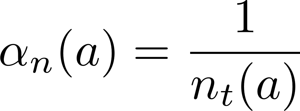
     \alpha_n(a) = \frac{1}{n_t(a)}
\end{align*}
\begin{align*}
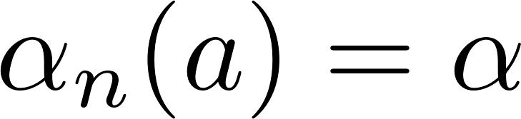
    \alpha_n(a) = \alpha 
\end{align*}

Sample-average method

(more suitable for stationary bandit)

Action-value function update equation

Weight-average method

(suitable for stationary and nonstationary bandit)
\begin{align*}
\alpha_n(a) = \frac{1}{n_t(a)}
\end{align*}
\begin{align*}
Q_{n+1}(a) = Q_n(a) + \alpha_n(a) \Big[ R_n - Q_n(a) \Big]
\end{align*}
\begin{align*}
\alpha_n(a) = \alpha
\end{align*}

Algorithms: Action-value methods

Greedy

UCB

Softmax

-greedy

Action-value update rule

Policies

\begin{align*}
Q_{n+1}(a) = Q_n(a) + \alpha_n(a) \Big[ R_n - Q_n(a) \Big]
\end{align*}

Method

Stochasticity

Exploration Strategy

Ability to Escape Local Optima

Greedy

𝜖-greedy

UCB

SoftMax

Algorithms: Summary

Method

Stochasticity

Exploration Strategy

Ability to Escape Local Optima

Greedy

Deterministic

𝜖-greedy

Stochastic

UCB

Deterministic

SoftMax

Stochastic

Algorithms: Summary

Method

Stochasticity

Exploration Strategy

Ability to Escape Local Optima

Greedy

Deterministic

No exploration

𝜖-greedy

Stochastic

Random actions with a small probability

UCB

Deterministic

Guided by uncertainty of action-value estimates

SoftMax

Stochastic

Probabilistic selection based on action-value

Algorithms: Summary

Method

Stochasticity

Exploration Strategy

Ability to Escape Local Optima

Greedy

Deterministic

No exploration

No (can get trapped in a suboptimal action)

𝜖-greedy

Stochastic

Random actions with a small probability

Yes (due to random exploration)

UCB

Deterministic

Guided by uncertainty of action-value estimates

Yes (due to uncertainty-based exploration)

SoftMax

Stochastic

Probabilistic selection based on action-value

Yes (assigns non-zero probability to all actions)

Algorithms: Summary

The multi-armed bandit problem

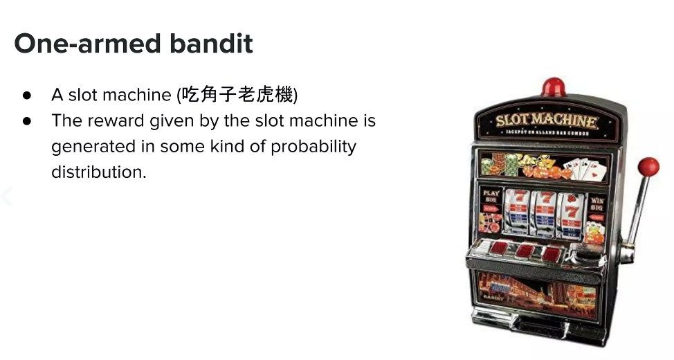
•You are in a casino with many slot machines.

•You will play 1000 times.

•Each time, you choose one machine.

•Your goal is to win as much money as possible.
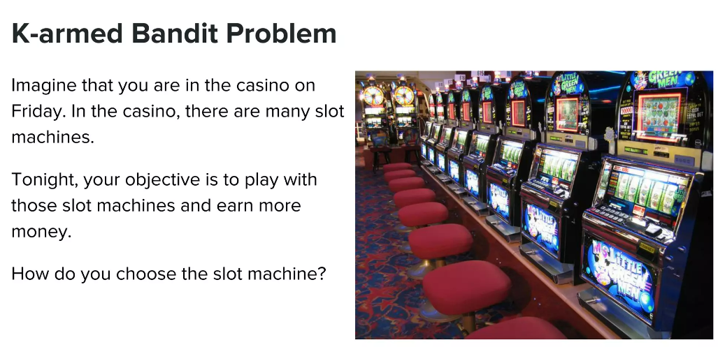
How do you choose which slot
machine to play each time?

Recap
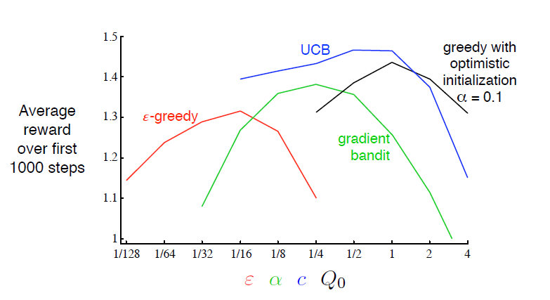
Parameter study of various bandit algorithms. Each point is the average reward obtained
over 1000 steps with a particular algorithm at a particular setting of its parameter.

See book’s page 42 for details.

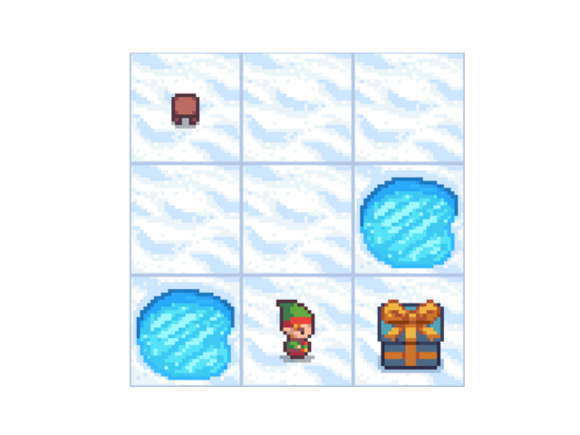
Frozen Lake game

How is this different from the bandit problem?
You will play this game 1000 times.

Your goal is to get the most points out of this experience.

You only know your position, the actions you can take, and the points
that you are receiving!

​

How do you choose your actions?

Frozen Lake game

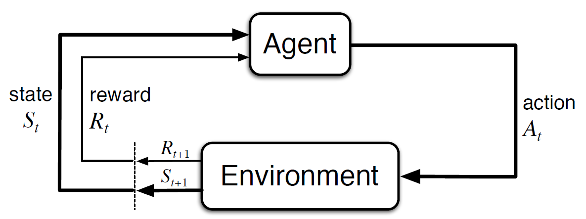
At each time-step , the agent is in state , takes an action,
receives a reward
, and transits to next-state

​

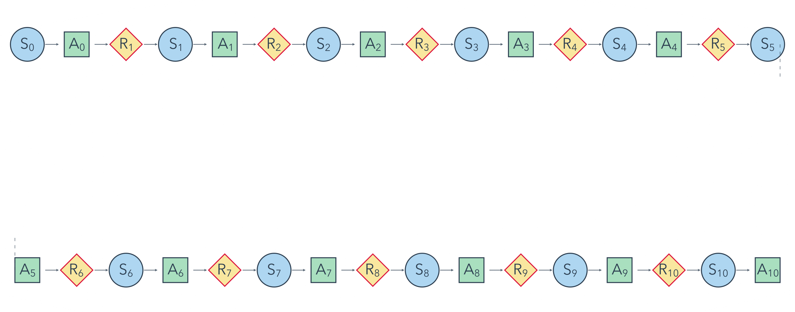
At each episode, we have a trajectory:

\begin{align*}
S_0, A_0, R_1, S_1, A_1, R_2, \ldots, S_t, A_t, R_{t+1}, \ldots, S_{T-1}, A_{T-1}, R_T, S_T
\end{align*}

where T is the time at the final state.

Is it possible to learn which sequences of actions will maximize
our total points after playing the game 1000 times by only
having access to the data generated from the trajectories?

The reward is the only information that tells us if our
actions were good or not! Is this enough?

Yes! According to the reward hypothesis!
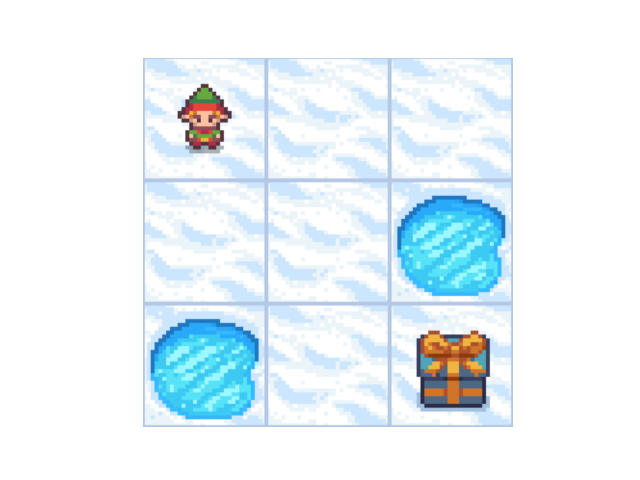
Frozen Lake Visualization.

Reward hypothesis

Any goal can be formalized as the outcome of maximizing a cumulative reward.

Reinforcement learning is based on the reward hypothesis:

Agent and Environment

Decision Maker

Frozen Lake game

Let’s understand and model the game.

What are the locations where the doll can be?

Which actions can the doll take?

After taking an action, how does the doll change its location?

Frozen Lake game

What are the locations where the doll can be?

Which actions can the doll take?

After taking an action, how does the doll change its location?

State Space =

Action Space = {up, down, left, right}

Transition function: Given state and action, provides the new state.

Frozen Lake game

Transition function: Given state and action, provides the new state.

The player may not always move in
the intended direction due to the
slippery nature of the frozen lake!

How can I represent this transitions mathematically?

State:

New State:

Action: right

State:

New State:

Action: right

Frozen Lake game

How can I represent this transitions mathematically?

State space

\begin{align*}
\mathcal{S} = \{s_1, \ldots, s_9\}
\end{align*}
\begin{align*}
S_t
\end{align*}

State random
variable at time t

Action space

\begin{align*}
\mathcal{A} = \{a_1, a_2, a_3, a_4\}
\end{align*}

up

down

left

right

\begin{align*}
A_t
\end{align*}

Action random
variable at time t

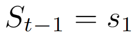
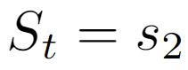
\begin{align*}
S_{t-1} = s_1
\end{align*}
\begin{align*}
S_t = s_2
\end{align*}
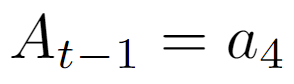
\begin{align*}
A_{t-1} = a_4
\end{align*}
\begin{align*}
Pr\{S_t = s_2|S_{t-1} = s_1, A_{t-1} = a_4\} = 0.90
\end{align*}
\begin{align*}
A_{t-1} = a_4
\end{align*}
\begin{align*}
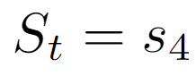
S_t = s_4
\end{align*}
\begin{align*}
S_{t-1} = s_1
\end{align*}
\begin{align*}
Pr\{S_t = s_4|S_{t-1} = s_1, A_{t-1} = a_4\} = 0.05
\end{align*}
\begin{align*}
p(s'|s,a) \doteq Pr\{S_t = s'|S_{t-1} = s, A_{t-1} = a\}
\end{align*}

Transition
function

Frozen Lake game

How can I represent this transitions mathematically?

\begin{align*}
p(s'|s,a) \doteq Pr\{S_t = s'|S_{t-1} = s, A_{t-1} = a\}
\end{align*}

Transition
function

State space

\begin{align*}
\mathcal{S} = \{s_1, \ldots, s_9\}
\end{align*}

Action space

\begin{align*}
\mathcal{A} = \{a_1, a_2, a_3, a_4\}
\end{align*}
\begin{align*}
p : \mathcal{S} \times \mathcal{A} \times \mathcal{S} \rightarrow [0, 1]
\end{align*}

What about the rewards?

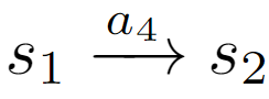
\begin{align*}
s_1 \xrightarrow{a_4} s_2
\end{align*}
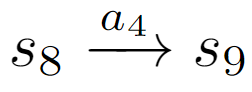
\begin{align*}
s_8 \xrightarrow{a_4} s_9
\end{align*}
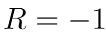
\begin{align*}
R = -1
\end{align*}
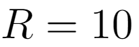
\begin{align*}
R = 10
\end{align*}

Random variable

Expected reward,
achieved on a transition
starting in (s, a)

\begin{align*}
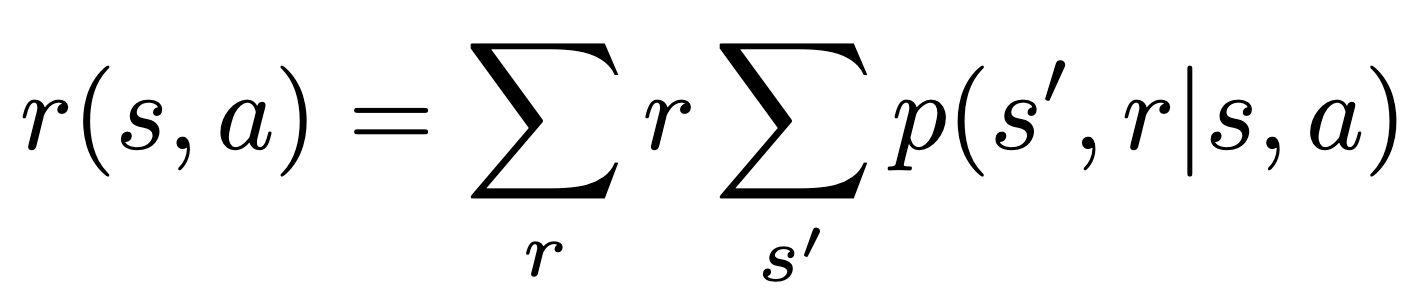
r(s,a) = \mathbb{E}[R_t|S_{t-1} = s, A_{t-1} = a]
\end{align*}
\begin{align*}
r : \mathcal{S} \times \mathcal{A} \rightarrow \mathbb{R}
\end{align*}

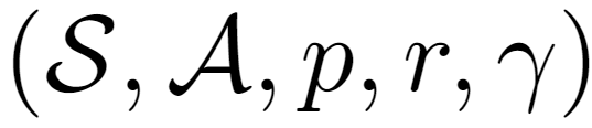
A Markov Decision Process (MDP) is a tuple

Markov Decision Process

\begin{align*}
(\mathcal{S}, \mathcal{A}, p, r, \gamma)
\end{align*}

Set of all
possible states

Set of all
possible actions

\begin{align*}
p(s'|s,a) \doteq Pr\{S_t = s'|S_{t-1} = s, A_{t-1} = a\}
\end{align*}
\begin{align*}
p : \mathcal{S} \times \mathcal{A} \times \mathcal{S} \rightarrow [0, 1]
\end{align*}

Probability of transitioning to , given a state and action .

Dynamics of the system.

Transition Function

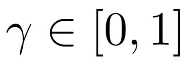
Discount factor

\begin{align*}
\gamma \in [0, 1]
\end{align*}

Expected reward, achieved on a
transition starting in (s, a)
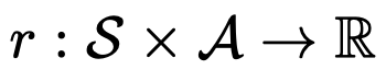
\begin{align*}
r : \mathcal{S} \times \mathcal{A} \rightarrow \mathbb{R}
\end{align*}

Markov Decision Process

A Markov Decision Process (MDP) is a tuple

\begin{align*}
(\mathcal{S}, \mathcal{A}, p, r, \gamma)
\end{align*}

Environment

Algorithm

MDP

A Markov Decision Process (MDP) is a tuple

\begin{align*}
(\mathcal{S}, \mathcal{A}, p, r, \gamma)
\end{align*}

Markov Decision Process

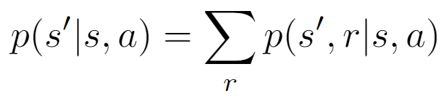
\begin{align*}
p(s', r|s, a) \doteq Pr\{S_t = s', R_t = r|S_{t-1} = s, A_{t-1} = a\}
\end{align*}
\begin{align*}
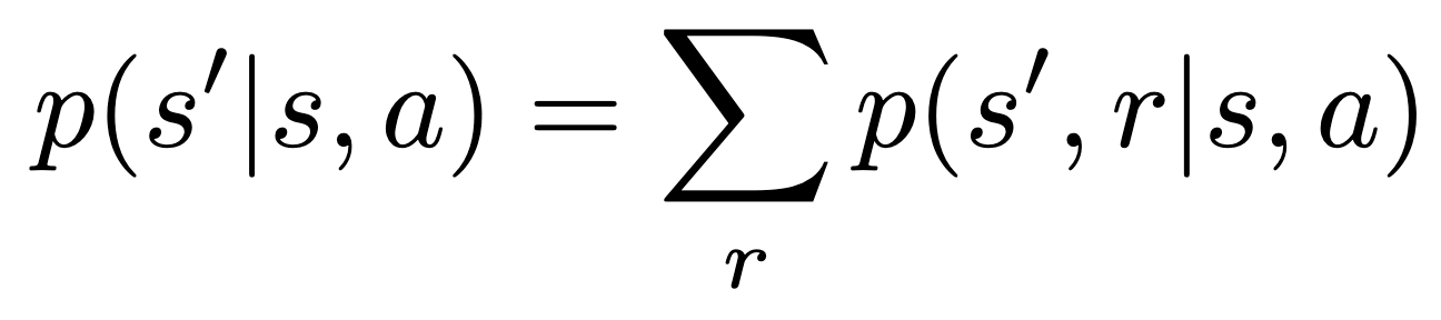
p(s'|s,a) = \sum_r p(s', r|s, a)
\end{align*}

If we define

then

\begin{align*}
\mathbb{E}[R_t|S_{t-1} = s, A_{t-1} = a] = \sum_r r \sum_{s'} p(s', r|s, a)
\end{align*}

Markov Property

The future is independent of the past given the present.

Define history as all previous
states, actions, and rewards.

\begin{align*}
h_{t-1} = \{S_1, \ldots, S_{t-1}, A_1, \ldots, A_{t-1}, R_1, \ldots, R_{t-1}\}
\end{align*}

In a Markov Decision Process all states are assumed to have the Markov property.

\begin{align*}
p(S_{t+1} = s'|S_t = s) = p(S_{t+1} = s'|h_{t-1}, S_t = s)
\end{align*}

Markov Property

➢The state captures all relevant information from the history.

➢Once the state is known, the history may be thrown away.

➢The state is a sufficient statistic of the past.

Markov Property

The future is independent of the past given the present.
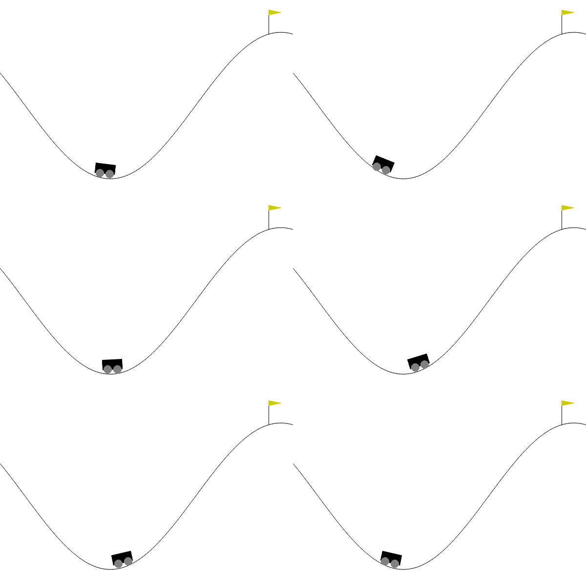
Mountain car

Observations

Position of the car

Markov Property

Screen Image
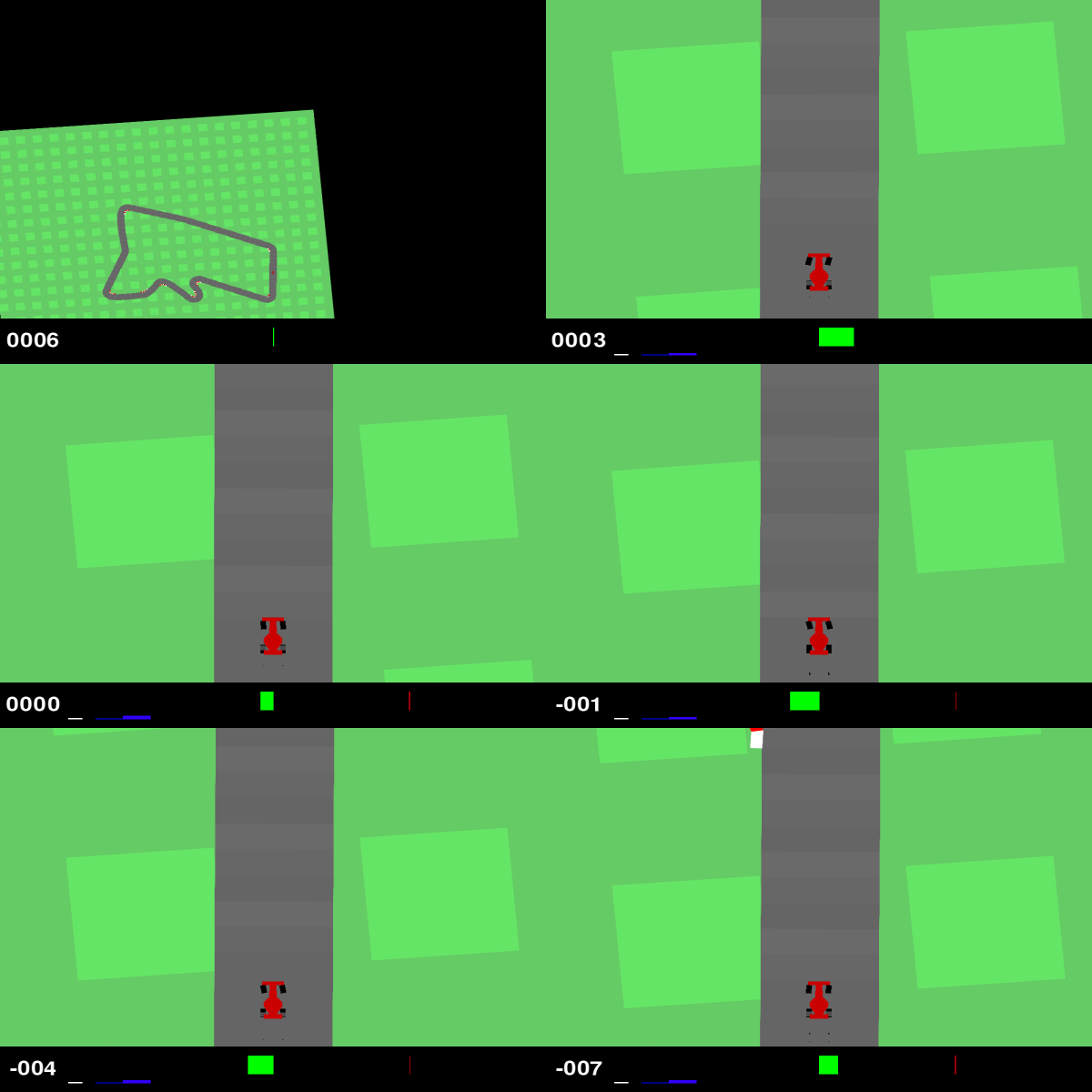
Car Racing

Observations

Markov Property

Sequence of 4 frames
of the screen Image

Frozen Lake

Observations

Markov
Property

Position of the doll

Position, velocity, and
acceleration of the car

Markov Property

The future is independent of the past given the present.

\begin{align*}
p(S_{t+1} = s'|S_t = s) = p(S_{t+1} = s'|h_{t-1}, S_t = s)
\end{align*}

Which of the following statements are true in a MDP?

\begin{align*}
p(S_{t+1} = s'|S_t = s, A_t = a) = p(S_{t+1} = s'|S_1, \ldots, S_{t-1}, S_t = s, A_t = a)
\end{align*}
\begin{align*}
p(S_{t+1} = s'|S_t = s, A_t = a) = p(S_{t+1} = s'|S_1, \ldots, S_{t-1}, S_t = s)
\end{align*}
\begin{align*}
p(R_{t+1} = r, S_{t+1} = s'|S_t = s) = p(R_{t+1} = r, S_{t+1} = s'|S_1, \ldots, S_{t-1}, S_t = s)
\end{align*}
\begin{align*}
p(S_{t+1} = s'|S_t = s, A_t = a) = p(S_{t+1} = s'|S_1, \ldots, S_{t-1}, A_1, \ldots, A_t = a, S_t = s)
\end{align*}

Partially Observable Environments

Partial observability: The observations are not Markovian

​

➢A robot with camera vision isn’t told its absolute location

​

➢A poker playing agent only observes public cards

​

Using the observation as state would not be Markovian

​

This is called a partially observable Markov decision process (POMDP)

​

The environment state can still be Markov, but the agent does not know it

​

We might still be able to construct an “artificial” MDP from a POMDP. This will not be
covered in this course
.

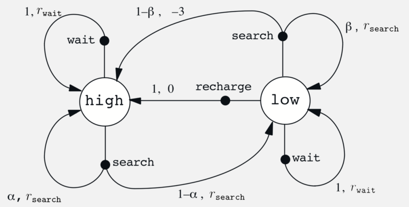
Example: cleaning robot

s

a

s‘

p(s’ | s, a)

r(s, a, s’ )

H

W

H

1

H

W

L

0

-

H

S

H

H

S

L

L

W

H

0

-

L

W

L

1

L

S

H

-3

L

S

L

L

re

H

1

0

L

re

L

0

-

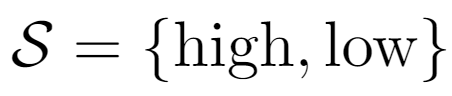
\begin{align*}
\mathcal{S} = \{\text{high}, \text{low}\}
\end{align*}

Example of a transition function

\begin{align*}
\mathcal{A}(\text{high}) = \{\text{wait}, \text{search}\}
\end{align*}
\begin{align*}
\mathcal{A}(\text{low}) = \{\text{wait}, \text{search}, \text{recharge}\}
\end{align*}
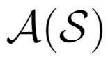
\begin{align*}
\mathcal{A}(\mathcal{S})
\end{align*}

Example: cleaning robot

s

a

s‘

p(s’ | s, a)

r(s, a, s’ )

H

W

H

1

H

W

L

0

-

H

S

H

H

S

L

L

W

H

0

-

L

W

L

1

L

S

H

-3

L

S

L

L

re

H

1

0

L

re

L

0

-

\begin{align*}
\mathcal{S} = \{\text{high}, \text{low}\}
\end{align*}

Example of a transition function

\begin{align*}
\mathcal{A}(\text{high}) = \{\text{wait}, \text{search}\}
\end{align*}
\begin{align*}
\mathcal{A}(\text{low}) = \{\text{wait}, \text{search}, \text{recharge}\}
\end{align*}
\begin{align*}
\mathcal{A}(\mathcal{S})
\end{align*}

Policy

\begin{align*}
\pi(a|s) \doteq Pr\{A_t = a|S_t = s\}
\end{align*}
\begin{align*}
\pi : \mathcal{S} \times \mathcal{A} \rightarrow [0, 1] \;\text{ for all }\; s \in \mathcal{S}, a \in \mathcal{A}(s)
\end{align*}

Policy is a mapping from states to probabilities of selecting each
possible action.

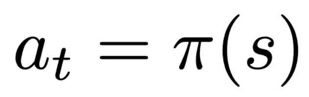
If a policy is deterministic, its representation can be simplified to:

\begin{align*}
\pi : \mathcal{S} \rightarrow \mathcal{A} \;\text{ for all }\; s \in \mathcal{S}, a \in \mathcal{A}(s)
\end{align*}
\begin{align*}
a_t = \pi(s)
\end{align*}
\begin{align*}
G_t \doteq R_{t+1} + R_{t+2} + \ldots + R_T = \sum_{k=0}^{T-t-1} R_{t+k+1}
\end{align*}

Returns

Is return a random variable?

Undiscounted return (episodic / finite horizon problems)

Return depends on rewards.

Are rewards random variables?
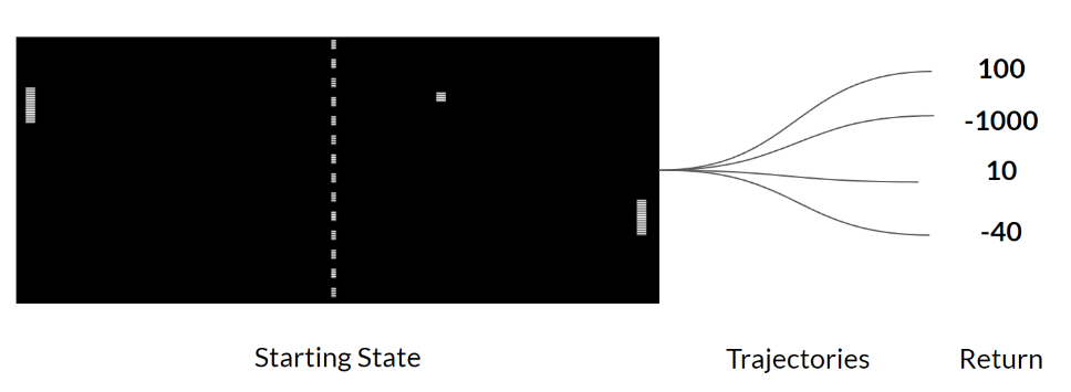
Each episode ends in a terminal state.

Final time step.

Return is a random variable that
depends on
MDP and policy!

\begin{align*}
G_t \doteq R_{t+1} + R_{t+2} + \ldots + R_T = \sum_{k=0}^{T-t-1} R_{t+k+1}
\end{align*}

Returns

Is return a random variable?

Undiscounted return (episodic / finite horizon problems)

Return depends on rewards.

Are rewards random variables?

Each episode ends in a terminal state.

Final time step.
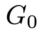
\begin{align*}
S_0, A_0, R_1, S_1, A_1, R_2, \ldots, S_{T-1}, A_{T-1}, R_T, S_T
\end{align*}
\begin{align*}
G_0
\end{align*}

Goal: Maximize what?

Expected return!

?

Goal of an RL agent

To find a target policy that maximizes the expected
return

Returns

Undiscounted return (episodic / finite horizon problems)

\begin{align*}
G_t \doteq R_{t+1} + R_{t+2} + \ldots + R_T = \sum_{k=0}^{T-t-1} R_{t+k+1}
\end{align*}

Discounted return (finite or infinite horizon problems)

\begin{align*}
G_t \doteq R_{t+1} + \gamma R_{t+2} + \gamma^2 R_{t+3} + \ldots = \sum_{k=0}^{\infty} \gamma^k R_{t+k+1}
\end{align*}
\begin{align*}
\gamma \in [0, 1]
\end{align*}

➢For , immediate rewards are more important than delayed rewards

➢ close to 0 leads to “myopic” evaluation

➢ close to 1 leads to “far-sighted” evaluation

Why discount?

Most Markov decision processes are discounted.

​

➢Problem specification:

➢Immediate rewards may actually be more valuable (e.g., earning interest)

➢Animal/human behavior shows preference for immediate reward

​

➢Solution side:

➢Mathematically convenient to discount rewards

➢Avoids infinite returns in cyclic Markov processes

​

Reward and discount together determine the goal!

Maximize expected return

Returns

Unified Notation for Episodic and Continuing Tasks
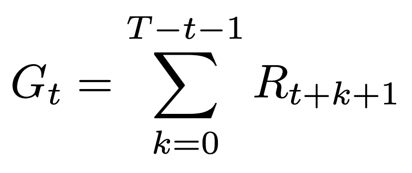
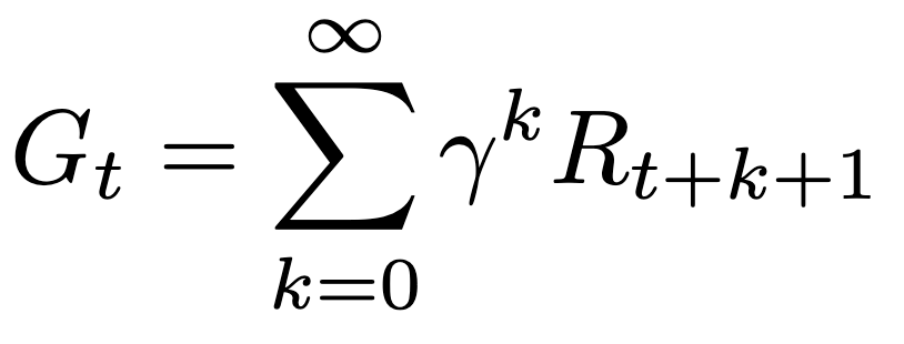
\begin{align*}
G_t = \sum_{k=0}^{T-t-1} R_{t+k+1}
\end{align*}

Episodic

\begin{align*}
G_t = \sum_{k=0}^{\infty} \gamma^k R_{t+k+1}
\end{align*}

Continuing

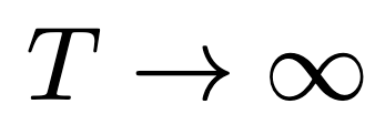
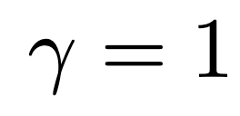
Absorbing state

\begin{align*}
T \rightarrow \infty
\end{align*}
\begin{align*}
\gamma = 1
\end{align*}

Unified Notation

Continuing

Episodic
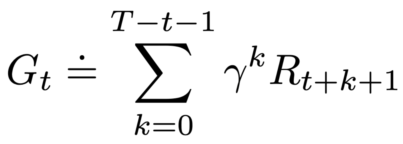
\begin{align*}
G_t \doteq \;\sum_{k=0}^{T-t-1}\; \gamma^k R_{t+k+1}
\end{align*}

Returns

Returns at successive time steps are related to each other
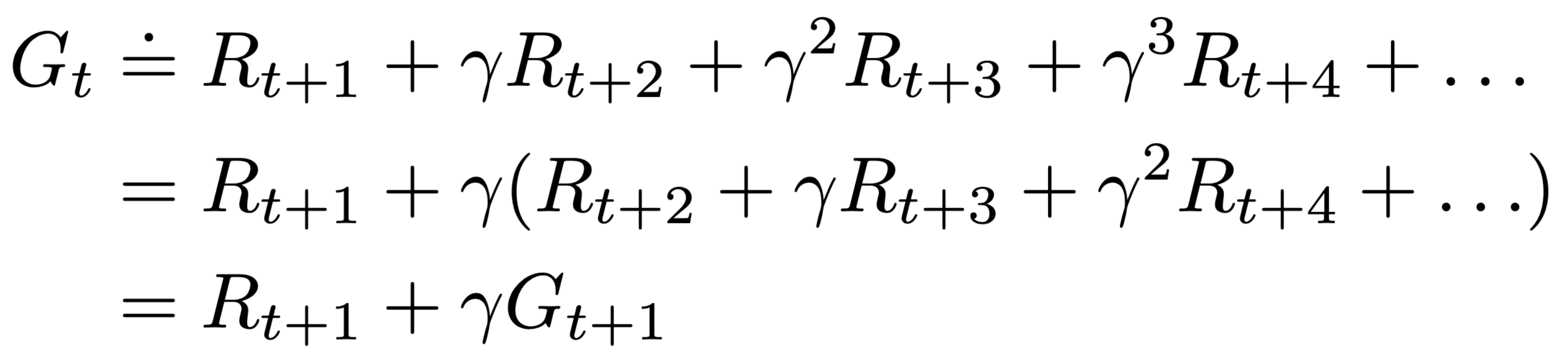
\begin{align*}
G_t &\doteq R_{t+1} + \gamma R_{t+2} + \gamma^2 R_{t+3} + \gamma^3 R_{t+4} + \ldots \\ &= R_{t+1} + \gamma(R_{t+2} + \gamma R_{t+3} + \gamma^2 R_{t+4} + \ldots) \\ &= R_{t+1} + \gamma G_{t+1}
\end{align*}
\begin{align*}
G_t &\doteq R_{t+1} + \gamma R_{t+2} + \gamma^2 R_{t+3} + \gamma^3 R_{t+4} + \ldots \\ &= R_{t+1} + \gamma(R_{t+2} + \gamma R_{t+3} + \gamma^2 R_{t+4} + \ldots) \\ &= R_{t+1} + \gamma G_{t+1}
\end{align*}
\begin{align*}
G_t &\doteq R_{t+1} + \gamma R_{t+2} + \gamma^2 R_{t+3} + \gamma^3 R_{t+4} + \ldots \\ &= R_{t+1} + \gamma(R_{t+2} + \gamma R_{t+3} + \gamma^2 R_{t+4} + \ldots) \\ &= R_{t+1} + \gamma G_{t+1}
\end{align*}

Returns: Gridworld Example

Gridworld with as terminal state.

State Space:

Action Space:

Transitions: Deterministic

Which policy is better?

Return with starting at:

Trajectory:

:

Returns: Gridworld Example

Gridworld with as terminal state.

State Space:

Action Space:

Transitions: Deterministic

Which policy is better?

Return with starting at:

:

Return with starting at:

:

Returns: Gridworld Example

Gridworld with as terminal state.

State Space:

Action Space:

Transitions: Deterministic

Which policy is better?

Return with starting at:

:

Return with starting at:

:

9

10

8

0

9

10

10

0

State-value function:

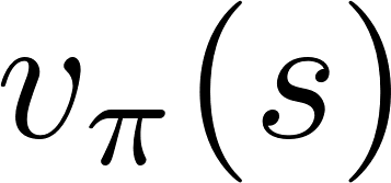
\begin{align*}
v_\pi(s) \doteq \mathbb{E}_\pi[G_t|S_t = s]
\end{align*}

Comparing policies

Goal of RL: To find a target policy that maximizes the expected return

\begin{align*}
v_\pi(s) \doteq \mathbb{E}_\pi[G_t|S_t = s]
\end{align*}

The state-value function gives the expected return when starting in state s, and
following the policy thereafter.

\begin{align*}
\pi \geq \pi' \iff v_\pi(s) \geq v_{\pi'}(s) \ , \text{ for all } s \in \mathcal{S}
\end{align*}

Value functions can be used to define a partial ordering over policies!

How can we evaluate how good the found policy is?

Comparing Policies: Ex1

Which policy is better?
\begin{align*}
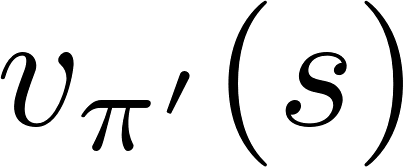
v_{\pi}(s)
\end{align*}
\begin{align*}
v_{\pi'}(s)
\end{align*}
\begin{align*}
\mathcal{S} = \{s_1, s_2, s_3, s_4 \}
\end{align*}
\begin{align*}
s_1 \qquad s_2 \qquad s_3 \qquad s_4
\end{align*}
\begin{align*}
s_1 \qquad s_2 \qquad s_3 \qquad s_4
\end{align*}
\begin{align*}
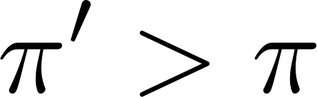
 v_{\pi'}(s) \geq v_{\pi}(s) \quad \forall  s \in \mathcal{S}
\end{align*}
\begin{align*}
\pi' > \pi
\end{align*}

Comparing Policies: Ex2

Which policy is better?

\begin{align*}
v_{\pi'}(s) > v_\pi(s) \quad \forall s \in \mathcal{S}
\end{align*}

Is

?

It is NOT defined
which policy is better.

\begin{align*}
s_1 \qquad s_2 \qquad s_3 \qquad s_4
\end{align*}
\begin{align*}
s_1 \qquad s_2 \qquad s_3 \qquad s_4
\end{align*}
\begin{align*}
\mathcal{S} = \{s_1, s_2, s_3, s_4 \}
\end{align*}
\begin{align*}
v_{\pi}(s)
\end{align*}
\begin{align*}
v_{\pi'}(s)
\end{align*}

Recursive relationships for the value functions
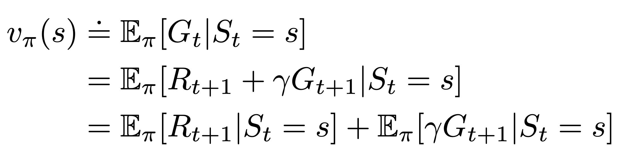
Write as a function of the value function in the next state

Transition:

Recursive relationships for the value functions
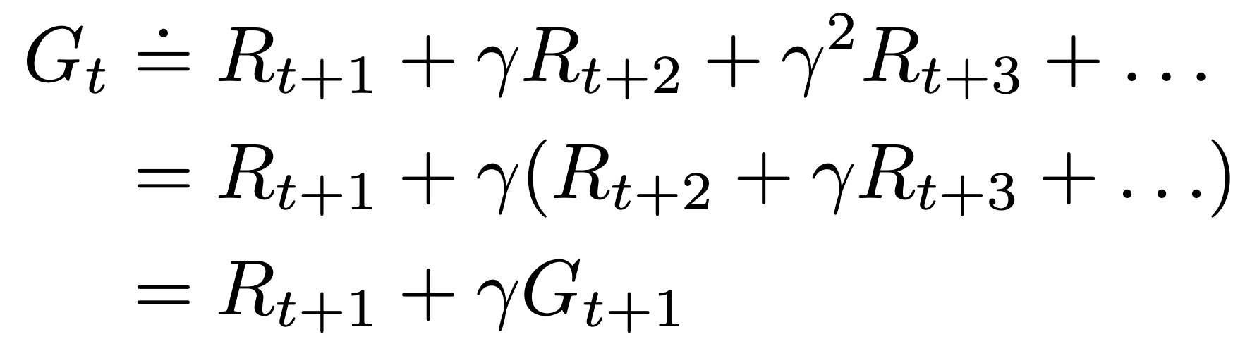
\begin{align*}
v_\pi(s) &\doteq \mathbb{E}_\pi[G_t|S_t = s] \\ &= \mathbb{E}_\pi[R_{t+1} + \gamma G_{t+1}|S_t = s] \\ &= \mathbb{E}_\pi[R_{t+1}|S_t = s] + \mathbb{E}_\pi[\gamma G_{t+1}|S_t = s]
\end{align*}
\begin{align*}
v_\pi(s) &\doteq \mathbb{E}_\pi[G_t|S_t = s] \\ &= \mathbb{E}_\pi[R_{t+1} + \gamma G_{t+1}|S_t = s] \\ &= \mathbb{E}_\pi[R_{t+1}|S_t = s] + \mathbb{E}_\pi[\gamma G_{t+1}|S_t = s]
\end{align*}
\begin{align*}
v_\pi(s) &\doteq \mathbb{E}_\pi[G_t|S_t = s] \\ &= \mathbb{E}_\pi[R_{t+1} + \gamma G_{t+1}|S_t = s] \\ &= \mathbb{E}_\pi[R_{t+1}|S_t = s] + \mathbb{E}_\pi[\gamma G_{t+1}|S_t = s]
\end{align*}
\begin{align*}
G_t &\doteq R_{t+1} + \gamma R_{t+2} + \gamma^2 R_{t+3} + \ldots \\ &= R_{t+1} + \gamma(R_{t+2} + \gamma R_{t+3} + \ldots) \\ &= R_{t+1} + \gamma G_{t+1}
\end{align*}
\begin{align*}
r(s,a) = \mathbb{E}[R_t|S_{t-1} = s, A_{t-1} = a]
\end{align*}
\begin{align*}
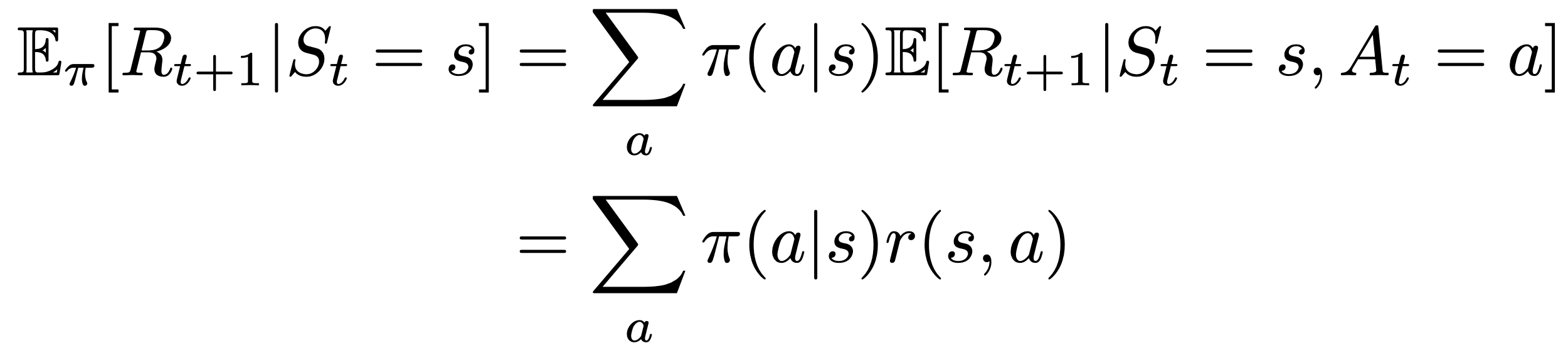
\mathbb{E}_\pi[R_{t+1}|S_t = s] &= \sum_a \pi(a|s) \mathbb{E}[R_{t+1}|S_t = s, A_t = a] \\ &= \sum_a \pi(a|s) r(s,a)
\end{align*}
\begin{align*}
\mathbb{E}_\pi[R_{t+1}|S_t = s] &= \sum_a \pi(a|s) \mathbb{E}[R_{t+1}|S_t = s, A_t = a] \\ &= \sum_a \pi(a|s) r(s,a)
\end{align*}
\begin{align*}
\mathbb{E}_\pi[R_{t+1}|S_t = s] &= \sum_a \pi(a|s) \mathbb{E}[R_{t+1}|S_t = s, A_t = a] \\ &= \sum_a \pi(a|s) r(s,a)
\end{align*}

Recursive relationships for the value functions

\begin{align*}
v_\pi(s) &\doteq \mathbb{E}_\pi[G_t|S_t = s] \\ &= \mathbb{E}_\pi[R_{t+1} + \gamma G_{t+1}|S_t = s] \\ &= \mathbb{E}_\pi[R_{t+1}|S_t = s] + \mathbb{E}_\pi[\gamma G_{t+1}|S_t = s]
\end{align*}
\begin{align*}
v_\pi(s) &\doteq \mathbb{E}_\pi[G_t|S_t = s] \\ &= \mathbb{E}_\pi[R_{t+1} + \gamma G_{t+1}|S_t = s] \\ &= \mathbb{E}_\pi[R_{t+1}|S_t = s] + \mathbb{E}_\pi[\gamma G_{t+1}|S_t = s]
\end{align*}
\begin{align*}
v_\pi(s) &\doteq \mathbb{E}_\pi[G_t|S_t = s] \\ &= \mathbb{E}_\pi[R_{t+1} + \gamma G_{t+1}|S_t = s] \\ &= \mathbb{E}_\pi[R_{t+1}|S_t = s] + \mathbb{E}_\pi[\gamma G_{t+1}|S_t = s]
\end{align*}
\begin{align*}
G_t &\doteq R_{t+1} + \gamma R_{t+2} + \gamma^2 R_{t+3} + \ldots \\ &= R_{t+1} + \gamma(R_{t+2} + \gamma R_{t+3} + \ldots) \\ &= R_{t+1} + \gamma G_{t+1}
\end{align*}
\begin{align*}
r(s,a) = \mathbb{E}[R_t|S_{t-1} = s, A_{t-1} = a]
\end{align*}
\begin{align*}
\mathbb{E}_\pi[R_{t+1}|S_t = s] &= \sum_a \pi(a|s) \mathbb{E}[R_{t+1}|S_t = s, A_t = a] \\ &= \sum_a \pi(a|s) r(s,a)
\end{align*}
\begin{align*}
\mathbb{E}_\pi[R_{t+1}|S_t = s] &= \sum_a \pi(a|s) \mathbb{E}[R_{t+1}|S_t = s, A_t = a] \\ &= \sum_a \pi(a|s) r(s,a)
\end{align*}

Recursive relationships for the value functions
\begin{align*}
v_\pi(s) &\doteq \mathbb{E}_\pi[G_t|S_t = s] \\ &= \mathbb{E}_\pi[R_{t+1} + \gamma G_{t+1}|S_t = s] \\ &= \mathbb{E}_\pi[R_{t+1}|S_t = s] + \mathbb{E}_\pi[\gamma G_{t+1}|S_t = s]
\end{align*}
\begin{align*}
v_\pi(s) &\doteq \mathbb{E}_\pi[G_t|S_t = s] \\ &= \mathbb{E}_\pi[R_{t+1} + \gamma G_{t+1}|S_t = s] \\ &= \mathbb{E}_\pi[R_{t+1}|S_t = s] + \mathbb{E}_\pi[\gamma G_{t+1}|S_t = s]
\end{align*}
\begin{align*}
G_t &\doteq R_{t+1} + \gamma R_{t+2} + \gamma^2 R_{t+3} + \ldots \\ &= R_{t+1} + \gamma(R_{t+2} + \gamma R_{t+3} + \ldots) \\ &= R_{t+1} + \gamma G_{t+1}
\end{align*}
\begin{align*}
r(s,a) = \mathbb{E}[R_t|S_{t-1} = s, A_{t-1} = a]
\end{align*}
\begin{align*}
v_\pi(s) &\doteq \mathbb{E}_\pi[G_t|S_t = s] \\ &= \mathbb{E}_\pi[R_{t+1} + \gamma G_{t+1}|S_t = s] \\ &= \mathbb{E}_\pi[R_{t+1}|S_t = s] + \mathbb{E}_\pi[\gamma G_{t+1}|S_t = s]
\end{align*}
\begin{align*}
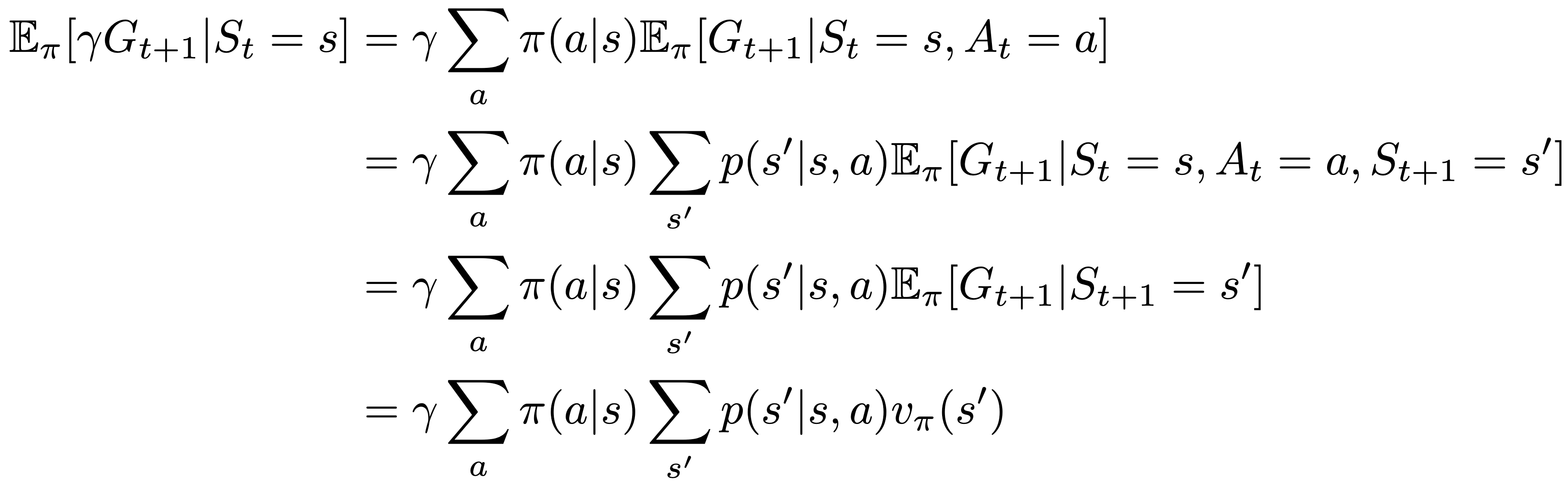
\mathbb{E}_\pi[\gamma G_{t+1}|S_t = s] &= \gamma\sum_{a}\pi(a|s)\mathbb{E}_\pi[G_{t+1}|S_t = s, A_t = a] \\ &= \gamma\sum_{a}\pi(a|s)\sum_{s'}p(s'|s,a)\mathbb{E}_\pi[G_{t+1}|S_t = s, A_t = a, S_{t+1} = s'] \\ &= \gamma\sum_{a}\pi(a|s)\sum_{s'}p(s'|s,a)\mathbb{E}_\pi[G_{t+1}|S_{t+1} = s'] \\ &= \gamma\sum_{a}\pi(a|s)\sum_{s'}p(s'|s,a)v_\pi(s')
\end{align*}
\begin{align*}
\mathbb{E}_\pi[\gamma G_{t+1}|S_t = s] &= \gamma\sum_{a}\pi(a|s)\mathbb{E}_\pi[G_{t+1}|S_t = s, A_t = a] \\ &= \gamma\sum_{a}\pi(a|s)\sum_{s'}p(s'|s,a)\mathbb{E}_\pi[G_{t+1}|S_t = s, A_t = a, S_{t+1} = s'] \\ &= \gamma\sum_{a}\pi(a|s)\sum_{s'}p(s'|s,a)\mathbb{E}_\pi[G_{t+1}|S_{t+1} = s'] \\ &= \gamma\sum_{a}\pi(a|s)\sum_{s'}p(s'|s,a)v_\pi(s')
\end{align*}
\begin{align*}
\mathbb{E}_\pi[\gamma G_{t+1}|S_t = s] &= \gamma\sum_{a}\pi(a|s)\mathbb{E}_\pi[G_{t+1}|S_t = s, A_t = a] \\ &= \gamma\sum_{a}\pi(a|s)\sum_{s'}p(s'|s,a)\mathbb{E}_\pi[G_{t+1}|S_t = s, A_t = a, S_{t+1} = s'] \\ &= \gamma\sum_{a}\pi(a|s)\sum_{s'}p(s'|s,a)\mathbb{E}_\pi[G_{t+1}|S_{t+1} = s'] \\ &= \gamma\sum_{a}\pi(a|s)\sum_{s'}p(s'|s,a)v_\pi(s')
\end{align*}
\begin{align*}
\mathbb{E}_\pi[\gamma G_{t+1}|S_t = s] &= \gamma\sum_{a}\pi(a|s)\mathbb{E}_\pi[G_{t+1}|S_t = s, A_t = a] \\ &= \gamma\sum_{a}\pi(a|s)\sum_{s'}p(s'|s,a)\mathbb{E}_\pi[G_{t+1}|S_t = s, A_t = a, S_{t+1} = s'] \\ &= \gamma\sum_{a}\pi(a|s)\sum_{s'}p(s'|s,a)\mathbb{E}_\pi[G_{t+1}|S_{t+1} = s'] \\ &= \gamma\sum_{a}\pi(a|s)\sum_{s'}p(s'|s,a)v_\pi(s')
\end{align*}
\begin{align*}
\mathbb{E}_\pi[\gamma G_{t+1}|S_t = s] &= \gamma\sum_{a}\pi(a|s)\mathbb{E}_\pi[G_{t+1}|S_t = s, A_t = a] \\ &= \gamma\sum_{a}\pi(a|s)\sum_{s'}p(s'|s,a)\mathbb{E}_\pi[G_{t+1}|S_t = s, A_t = a, S_{t+1} = s'] \\ &= \gamma\sum_{a}\pi(a|s)\sum_{s'}p(s'|s,a)\mathbb{E}_\pi[G_{t+1}|S_{t+1} = s'] \\ &= \gamma\sum_{a}\pi(a|s)\sum_{s'}p(s'|s,a)v_\pi(s')
\end{align*}
\begin{align*}
\mathbb{E}_\pi[R_{t+1}|S_t = s] &= \sum_a \pi(a|s) \mathbb{E}[R_{t+1}|S_t = s, A_t = a] \\ &= \sum_a \pi(a|s) r(s,a)
\end{align*}
\begin{align*}
\mathbb{E}_\pi[R_{t+1}|S_t = s] &= \sum_a \pi(a|s) \mathbb{E}[R_{t+1}|S_t = s, A_t = a] \\ &= \sum_a \pi(a|s) r(s,a)
\end{align*}
\begin{align*}
v_\pi(s') = \mathbb{E}_\pi[G_{t+1}|S_{t+1} = s']
\end{align*}

Markov Property

Recursive relationships for the value functions
\begin{align*}
v_\pi(s) &\doteq \mathbb{E}_\pi[G_t|S_t = s] \\ &= \mathbb{E}_\pi[R_{t+1} + \gamma G_{t+1}|S_t = s] \\ &= \mathbb{E}_\pi[R_{t+1}|S_t = s] + \mathbb{E}_\pi[\gamma G_{t+1}|S_t = s]
\end{align*}
\begin{align*}
v_\pi(s) &\doteq \mathbb{E}_\pi[G_t|S_t = s] \\ &= \mathbb{E}_\pi[R_{t+1} + \gamma G_{t+1}|S_t = s] \\ &= \mathbb{E}_\pi[R_{t+1}|S_t = s] + \mathbb{E}_\pi[\gamma G_{t+1}|S_t = s]
\end{align*}
\begin{align*}
G_t &\doteq R_{t+1} + \gamma R_{t+2} + \gamma^2 R_{t+3} + \ldots \\ &= R_{t+1} + \gamma(R_{t+2} + \gamma R_{t+3} + \ldots) \\ &= R_{t+1} + \gamma G_{t+1}
\end{align*}
\begin{align*}
r(s,a) = \mathbb{E}[R_t|S_{t-1} = s, A_{t-1} = a]
\end{align*}
\begin{align*}
v_\pi(s) &\doteq \mathbb{E}_\pi[G_t|S_t = s] \\ &= \mathbb{E}_\pi[R_{t+1} + \gamma G_{t+1}|S_t = s] \\ &= \mathbb{E}_\pi[R_{t+1}|S_t = s] + \mathbb{E}_\pi[\gamma G_{t+1}|S_t = s]
\end{align*}
\begin{align*}
\mathbb{E}_\pi[\gamma G_{t+1}|S_t = s] &= \gamma\sum_{a}\pi(a|s)\mathbb{E}_\pi[G_{t+1}|S_t = s, A_t = a] \\ &= \gamma\sum_{a}\pi(a|s)\sum_{s'}p(s'|s,a)\mathbb{E}_\pi[G_{t+1}|S_t = s, A_t = a, S_{t+1} = s'] \\ &= \gamma\sum_{a}\pi(a|s)\sum_{s'}p(s'|s,a)\mathbb{E}_\pi[G_{t+1}|S_{t+1} = s'] \\ &= \gamma\sum_{a}\pi(a|s)\sum_{s'}p(s'|s,a)v_\pi(s')
\end{align*}
\begin{align*}
\mathbb{E}_\pi[\gamma G_{t+1}|S_t = s] &= \gamma\sum_{a}\pi(a|s)\mathbb{E}_\pi[G_{t+1}|S_t = s, A_t = a] \\ &= \gamma\sum_{a}\pi(a|s)\sum_{s'}p(s'|s,a)\mathbb{E}_\pi[G_{t+1}|S_t = s, A_t = a, S_{t+1} = s'] \\ &= \gamma\sum_{a}\pi(a|s)\sum_{s'}p(s'|s,a)\mathbb{E}_\pi[G_{t+1}|S_{t+1} = s'] \\ &= \gamma\sum_{a}\pi(a|s)\sum_{s'}p(s'|s,a)v_\pi(s')
\end{align*}
\begin{align*}
\mathbb{E}_\pi[R_{t+1}|S_t = s] &= \sum_a \pi(a|s) \mathbb{E}[R_{t+1}|S_t = s, A_t = a] \\ &= \sum_a \pi(a|s) r(s,a)
\end{align*}
\begin{align*}
\mathbb{E}_\pi[R_{t+1}|S_t = s] &= \sum_a \pi(a|s) \mathbb{E}[R_{t+1}|S_t = s, A_t = a] \\ &= \sum_a \pi(a|s) r(s,a)
\end{align*}
\begin{align*}
v_\pi(s) = \sum_a \pi(a|s)\Big(r(s,a) + \gamma \sum_{s'} p(s'|s,a) v_\pi(s')\Big)
\end{align*}

Bellman expectation equation for the state-value function

Recursive relationships for the value functions

\begin{align*}
v_\pi(s) = \sum_a \pi(a|s)\Big(r(s,a) + \gamma \sum_{s'} p(s'|s,a) v_\pi(s')\Big)
\end{align*}

Bellman Expectation equation for the state-value function

Alternatively

\begin{align*}
v_\pi(s) = \sum_a \pi(a|s) \sum_r \sum_{s'} p(s', r|s, a)\Big(r + \gamma v_\pi(s')\Big)
\end{align*}
\begin{align*}
r(s,a) = \sum_r r \sum_{s'} p(s', r|s, a)
\end{align*}
\begin{align*}
p(s'|s,a) = \sum_r p(s', r|s, a)
\end{align*}

Bellman Expectation equation

\begin{align*}
v_\pi(s) = \sum_a \pi(a|s)\Big(r(s,a) + \gamma \sum_{s'} p(s'|s,a) v_\pi(s')\Big)
\end{align*}

Bellman Expectation equation for the state-value function

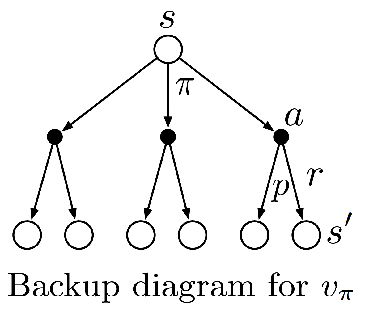
➢ and are state values to be calculated. Bootstrapping!

​

➢ is a given policy. Solving the equation is called policy evaluation.

​

➢ represents the dynamics of the MDP.

Backup diagram
\begin{align*}
v_\pi(s) = \sum_a \pi(a|s) \sum_r \sum_{s'} p(s', r|s, a)\Big(r + \gamma v_\pi(s')\Big)
\end{align*}

Returns: Gridworld Example

Gridworld with as terminal state.

State Space:

Action Space:

Transitions: Deterministic

9

10

8

0

\begin{align*}
q_\pi(s,a) \doteq \mathbb{E}_\pi[G_t|S_t = s, A_t = a]
\end{align*}

(state-)action value function

Returns: Gridworld Example

Gridworld with as terminal state.

State Space:

Action Space:

Transitions: Deterministic

9

10

8

0

\begin{align*}
q_\pi(s,a) \doteq \mathbb{E}_\pi[G_t|S_t = s, A_t = a]
\end{align*}

(state-)action value function

9

10

8

0

0

0

0

Returns: Gridworld Example

Gridworld with as terminal state.

State Space:

Action Space:

Transitions: Deterministic

9

10

8

0

\begin{align*}
q_\pi(s,a) \doteq \mathbb{E}_\pi[G_t|S_t = s, A_t = a]
\end{align*}

(state-)action value function

9

10

8

0

0

0

0

7

Value Functions

\begin{align*}
v_\pi(s) \doteq \mathbb{E}_\pi[G_t|S_t = s]
\end{align*}

The state-value function gives the long-term value of state s

\begin{align*}
q_\pi(s,a) \doteq \mathbb{E}_\pi[G_t|S_t = s, A_t = a]
\end{align*}

We can define the (state-)action value function
How are they connected?

Value Functions

\begin{align*}
v_\pi(s) \doteq \mathbb{E}_\pi[G_t|S_t = s]
\end{align*}
\begin{align*}
q_\pi(s,a) \doteq \mathbb{E}_\pi[G_t|S_t = s, A_t = a]
\end{align*}

We can define the (state-)action value function

\begin{align*}
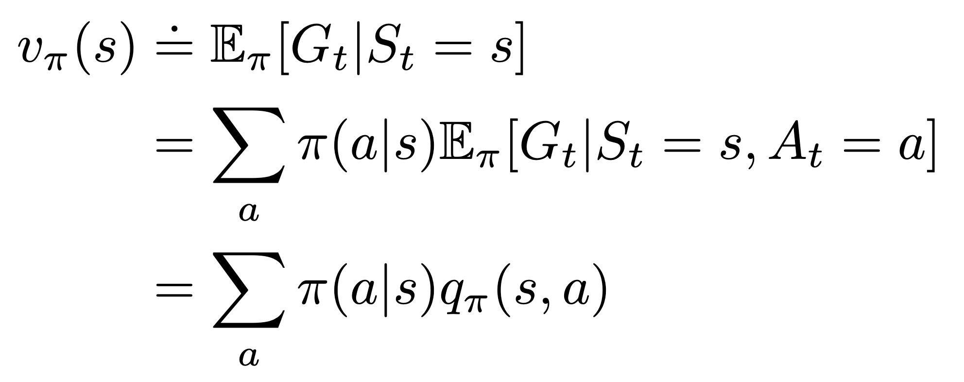
v_\pi(s) &\doteq \mathbb{E}_\pi[G_t|S_t = s] \\ &= \sum_{a}\pi(a|s)\mathbb{E}_\pi[G_t|S_t = s, A_t = a] \\ &= \sum_{a}\pi(a|s)q_\pi(s,a)
\end{align*}

Note that:

\begin{align*}
v_\pi(s) &\doteq \mathbb{E}_\pi[G_t|S_t = s] \\ &= \sum_{a}\pi(a|s)\mathbb{E}_\pi[G_t|S_t = s, A_t = a] \\ &= \sum_{a}\pi(a|s)q_\pi(s,a)
\end{align*}
\begin{align*}
v_\pi(s) &\doteq \mathbb{E}_\pi[G_t|S_t = s] \\ &= \sum_{a}\pi(a|s)\mathbb{E}_\pi[G_t|S_t = s, A_t = a] \\ &= \sum_{a}\pi(a|s)q_\pi(s,a)
\end{align*}
\begin{align*}
= \mathbb{E}[q_\pi(S_t, A_t)|S_t = s, A_t \sim \pi]
\end{align*}

The state-value function gives the long-term value of state s

\begin{align*}
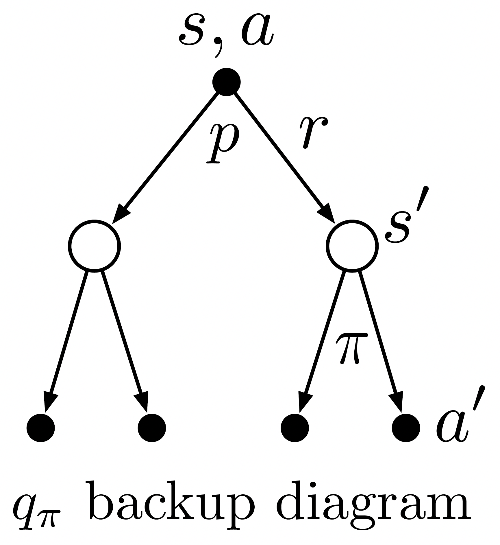
q_\pi(s,a) = \sum_r \sum_{s'} p(s', r|s, a)\Big(r + \gamma \sum_{a'} \pi(a'|s') q_\pi(s', a')\Big)
\end{align*}

Backup diagram

Try to prove it at home!

\begin{align*}
\mathcal{M} = (\mathcal{S}, \mathcal{A}, p, r, \gamma)
\end{align*}

Given an MDP, for any policy , the value functions
obey the following expectations equations:

Bellman Expectation Equations

Theorem

\begin{align*}
q_\pi(s,a) = r(s,a) + \gamma \sum_{s'} p(s'|s,a) \sum_{a'} \pi(a'|s') q_\pi(s', a')
\end{align*}
\begin{align*}
v_\pi(s) = \sum_a \pi(a|s)\Big(r(s,a) + \gamma \sum_{s'} p(s'|s,a) v_\pi(s')\Big)
\end{align*}
\begin{align*}
q_*(s,a) \doteq \max_\pi q_\pi(s,a)
\end{align*}
\begin{align*}
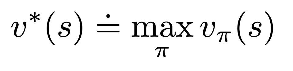
v_*(s) \doteq \max_\pi v_\pi(s)
\end{align*}

Optimal action-value function

is the maximum action-value function over all policies

Optimal state-value function

is the maximum state-value function over all policies

Optimal Value Function

Definition (Optimal value functions)

The optimal value function specifies the best possible performance in the MDP

An MDP is “solved” when we know the optimal value function

Optimal Policy

Define a partial ordering over policies

\begin{align*}
\pi \geq \pi' \iff v_\pi(s) \geq v_{\pi'}(s) \ , \text{ for all } s \in \mathcal{S}
\end{align*}

Theorem (Optimal Policies)

For any Markov decision process

There exist an optimal policy that is better than or equal to all other policies
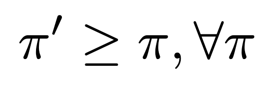
\begin{align*}
\pi' \geq \pi, \forall \pi
\end{align*}

(There can be more than one such optimal policy.)

All optimal policies achieve the optimal state-value function
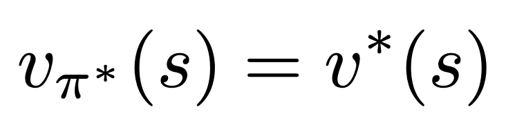
\begin{align*}
v_{\pi_*}(s) = v_*(s)
\end{align*}

All optimal policies achieve the optimal action-value function

\begin{align*}
q_{\pi_*}(s, a) = q_*(s, a)
\end{align*}

Finding an Optimal Policy

An optimal policy can be found by maximizing (greedy) over
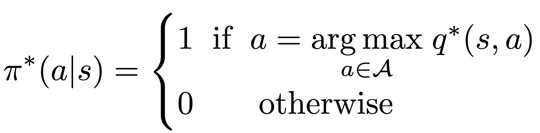
\begin{align*}
\pi_*(a|s) = \begin{cases} 1 \;\; \text{if} \;\; a = \underset{a \in \mathcal{A}}{\arg\max}\, q_*(s,a) \\ 0 \qquad\quad \text{otherwise} \end{cases}
\end{align*}

➢There is always a deterministic optimal policy for any MDP

➢If we know , we immediately have the optimal policy

➢There can be multiple optimal policies

➢If multiple actions maximize , we can just pick any of these (including stochastically)

Bellman Optimality equations
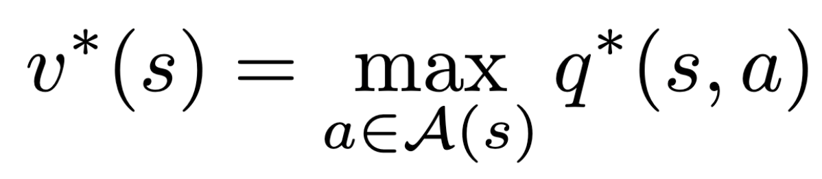
\begin{align*}
v_*(s) = \max_{a \in \mathcal{A}(s)} q_*(s,a)
\end{align*}
\begin{align*}
q_*(s,a) = \mathbb{E}[R_{t+1} + \gamma v_*(S_{t+1})|S_t = s, A_t = a]
\end{align*}
\begin{align*}
\pi_*(a|s) = \begin{cases} 1 \;\; \text{if} \;\; a = \underset{a \in \mathcal{A}}{\arg\max}\, q_*(s,a) \\ 0 \qquad\quad \text{otherwise} \end{cases}
\end{align*}

Bellman Optimality equations

\begin{align*}
v_*(s) = \max_{a \in \mathcal{A}(s)} q_*(s,a)
\end{align*}
\begin{align*}
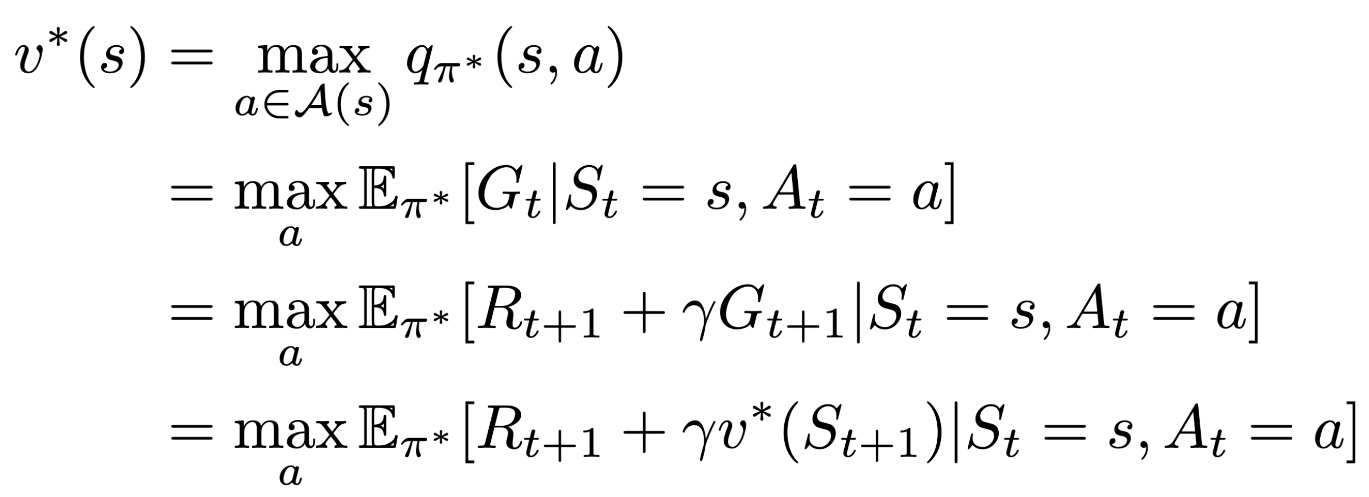
v_*(s) &= \max_{a\in\mathcal{A}(s)}\, q_{\pi_*}(s,a) \\ &= \max_{a}\mathbb{E}_{\pi_*}[G_t|S_t = s, A_t = a] \\ &= \max_{a}\mathbb{E}_{\pi_*}[R_{t+1} + \gamma G_{t+1}|S_t = s, A_t = a] \\ &= \max_{a}\mathbb{E}_{\pi_*}[R_{t+1} + \gamma v_*(S_{t+1})|S_t = s, A_t = a]
\end{align*}
\begin{align*}
v_*(s) &= \max_{a\in\mathcal{A}(s)}\, q_{\pi_*}(s,a) \\ &= \max_{a}\mathbb{E}_{\pi_*}[G_t|S_t = s, A_t = a] \\ &= \max_{a}\mathbb{E}_{\pi_*}[R_{t+1} + \gamma G_{t+1}|S_t = s, A_t = a] \\ &= \max_{a}\mathbb{E}_{\pi_*}[R_{t+1} + \gamma v_*(S_{t+1})|S_t = s, A_t = a]
\end{align*}
\begin{align*}
v_*(s) &= \max_{a\in\mathcal{A}(s)}\, q_{\pi_*}(s,a) \\ &= \max_{a}\mathbb{E}_{\pi_*}[G_t|S_t = s, A_t = a] \\ &= \max_{a}\mathbb{E}_{\pi_*}[R_{t+1} + \gamma G_{t+1}|S_t = s, A_t = a] \\ &= \max_{a}\mathbb{E}_{\pi_*}[R_{t+1} + \gamma v_*(S_{t+1})|S_t = s, A_t = a]
\end{align*}

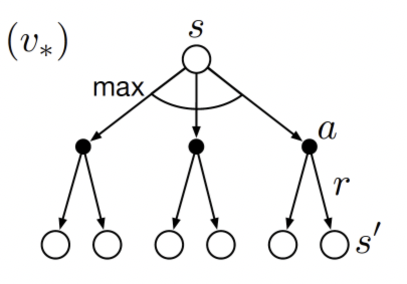
Bellman Optimality equations

\begin{align*}
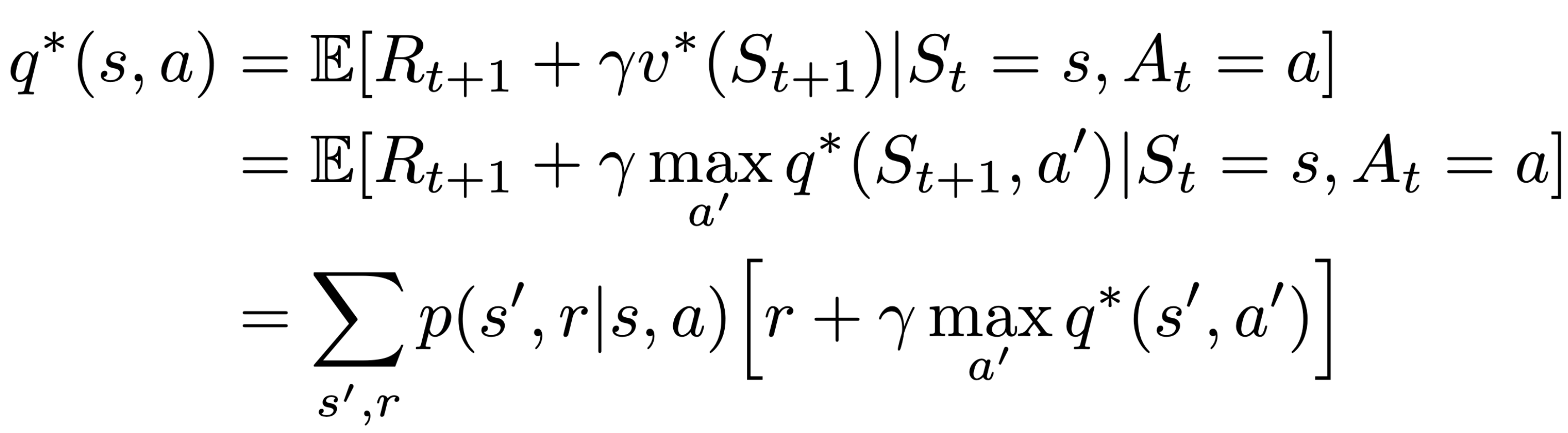
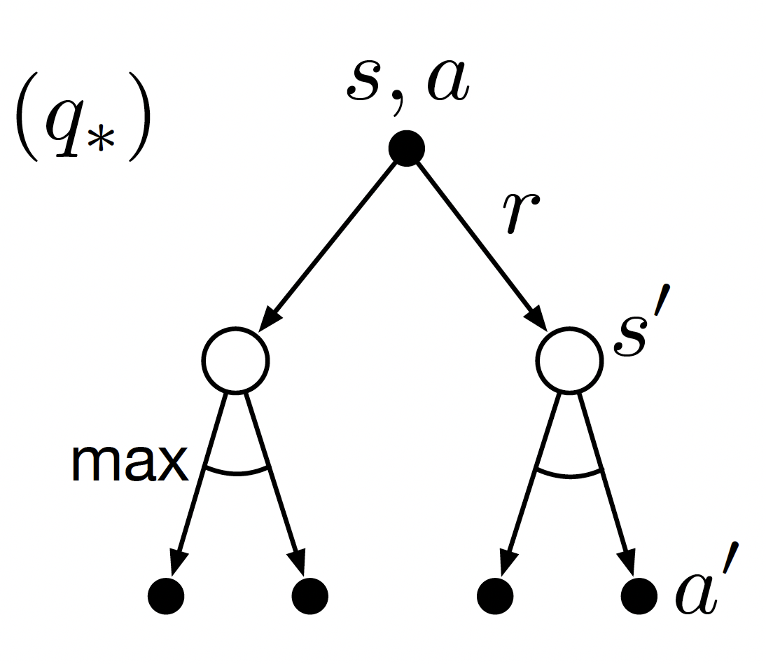
q_*(s,a) &= \mathbb{E}[R_{t+1} + \gamma v_*(S_{t+1})|S_t = s, A_t = a] \\ &= \mathbb{E}[R_{t+1} + \gamma\max_{a'}q_*(S_{t+1},a')|S_t = s, A_t = a] \\ &= \sum_{s',r}p(s',r|s,a)\Big[r + \gamma\max_{a'}q_*(s',a')\Big]
\end{align*}
\begin{align*}
v_*(s) = \max_{a \in \mathcal{A}(s)} q_*(s,a)
\end{align*}
\begin{align*}
q_*(s,a) &= \mathbb{E}[R_{t+1} + \gamma v_*(S_{t+1})|S_t = s, A_t = a] \\ &= \mathbb{E}[R_{t+1} + \gamma\max_{a'}q_*(S_{t+1},a')|S_t = s, A_t = a] \\ &= \sum_{s',r}p(s',r|s,a)\Big[r + \gamma\max_{a'}q_*(s',a')\Big]
\end{align*}

Bellman Equations

(Reminder) Greedy on = Optimal Policy

An optimal policy can be found
by maximizing (greedy) over

\begin{align*}
\pi_*(a|s) = \begin{cases} 1 \;\; \text{if} \;\; a = \underset{a \in \mathcal{A}}{\arg\max}\, q_*(s,a) \\ 0 \qquad\quad \text{otherwise} \end{cases}
\end{align*}

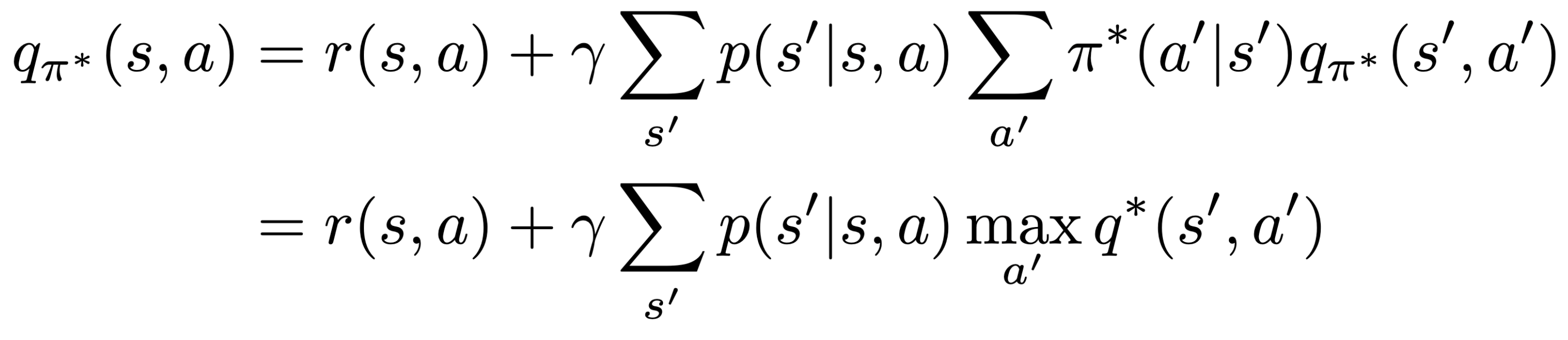
Applying the Bellman equation:

\begin{align*}
q_{\pi_*}(s,a) &= r(s,a) + \gamma\sum_{s'}p(s'|s,a)\sum_{a'}\pi_*(a'|s')q_{\pi_*}(s',a') \\ &= r(s,a) + \gamma\sum_{s'}p(s'|s,a)\max_{a'}q_*(s',a')
\end{align*}
\begin{align*}
q_{\pi_*}(s,a) &= r(s,a) + \gamma\sum_{s'}p(s'|s,a)\sum_{a'}\pi_*(a'|s')q_{\pi_*}(s',a') \\ &= r(s,a) + \gamma\sum_{s'}p(s'|s,a)\max_{a'}q_*(s',a')
\end{align*}
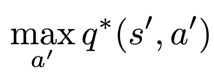
\begin{align*}
\max_{a'} q_*(s', a')
\end{align*}

Given an MDP, the optimal value functions obey the
following expectations equations:

Bellman Optimality Equations

Theorem

\begin{align*}
q_*(s,a) = r(s,a) + \gamma \sum_{s'} p(s'|s,a) \max_{a'} q_*(s', a')
\end{align*}
\begin{align*}
v_*(s) = \max_a \Big( r(s,a) + \gamma \sum_{s'}p(s'|s,a) v_* (s') \Big)
\end{align*}
\begin{align*}
\mathcal{M} = (\mathcal{S}, \mathcal{A}, p, r, \gamma)
\end{align*}

There can be no policy with a higher value than

\begin{align*}
v_{\pi}(s) = \max_{\pi} v_{\pi}(s),  \forall s \in \mathcal{S}
\end{align*}

Problems in RL

Estimating or

Policy evaluation / Prediction

Given a policy, what is my expected return under that behavior?

Given this treatment protocol/trading strategy, what is my expected return?

Estimating or

Control, because can be used for policy optimization

What is the optimal way of behaving? What is the optimal value function?

What is the optimal treatment? What is the optimal control policy to minimize time, fuel consumption, etc?

Exercise

Consider the following MDP:

➢ for all transitions that end up in , and for all other transitions.

What is ?
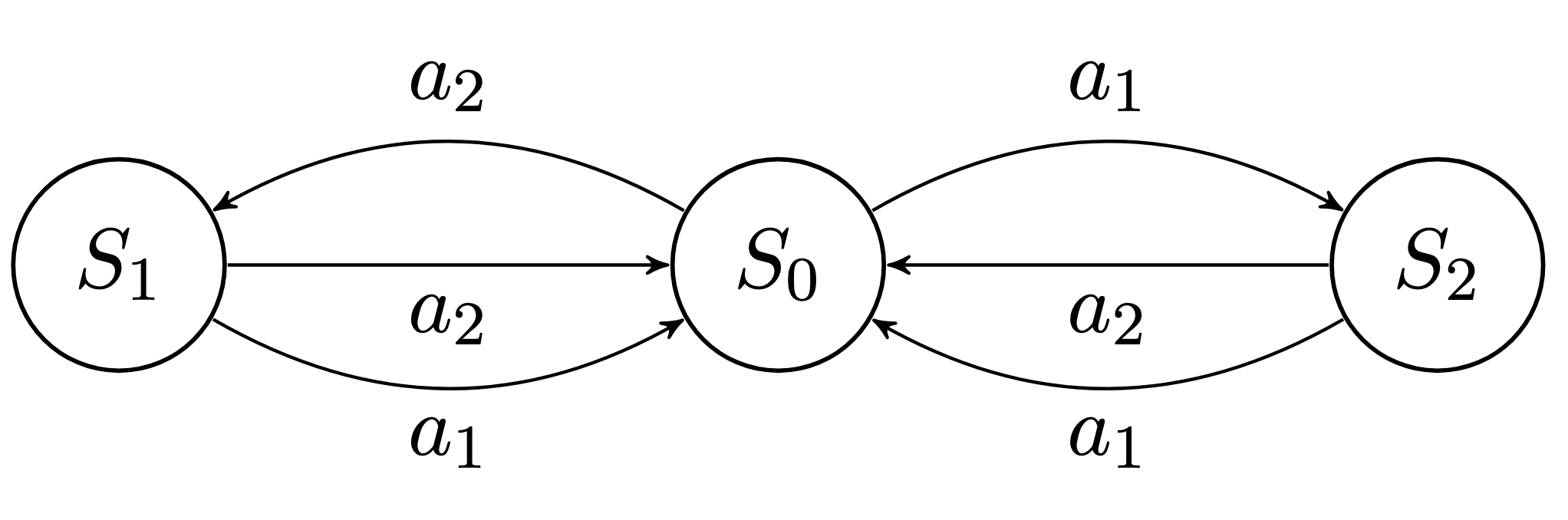
➢Actions have a 0.9 probability of success and with 0.1 probability we remain in the same state.

➢Consider a discount of .

\begin{align*}
v_{\pi}(s) = \sum_a \pi(a|s) \Big(r(s,a) + \gamma \sum_{s'}p(s'|s,a) v_{\pi}(s')\Big)
\end{align*}
\begin{align*}
v_\pi(s) & =\underbrace{\sum_a \pi(a \mid s) \sum_{s^{\prime}, r} p(s^{\prime}, r \mid s, a) r}_{r^\pi}+\gamma\underbrace{ \sum_a \pi(a \mid s) \sum_{s^{\prime}} p\left(s^{\prime} \mid s_i, a\right)}_{P^\pi} v_{\pi}\left(s^{\prime}\right) 
\end{align*}

➢ for all transitions that end up in , and for all other transitions.

What is ?

➢Actions have a 0.9 probability of success and with 0.1 probability we remain in the same state.

\begin{align*}
v_\pi(s) & =\underbrace{\sum_a \pi(a \mid s) \sum_{s^{\prime}, r} p(s^{\prime}, r \mid s, a) r}_{r^\pi}+\gamma\underbrace{ \sum_a \pi(a \mid s) \sum_{s^{\prime}} p\left(s^{\prime} \mid s_i, a\right)}_{P^\pi} v_{\pi}\left(s^{\prime}\right) 
\end{align*}
\begin{align*}
r_0^\pi  =\pi\left(a_1 \mid s_0\right)\left[p\left(s_2,-1 \mid s_0, a_1\right)(-1)+p\left(s_1,r \mid s_0, a_1\right)r+p\left(s_0, 0 \mid s_0, a_1\right) \cdot 0\right] 
\end{align*}
\begin{align*}
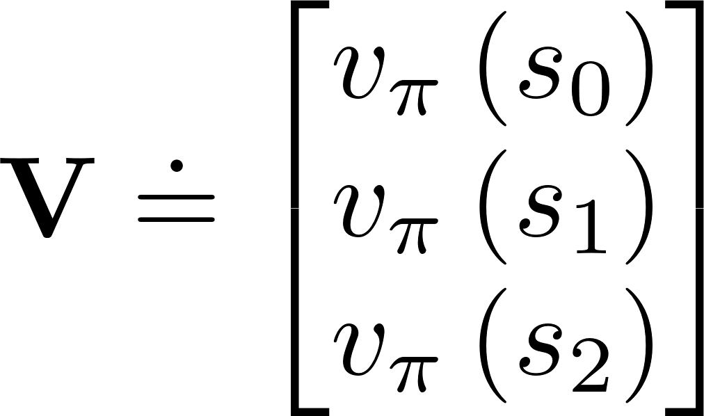
    \mathbf{V} \doteq \begin{bmatrix}
    v_\pi\left(s_0\right) \\
    v_\pi\left(s_1\right) \\
    v_\pi\left(s_2\right)
    \end{bmatrix}
\end{align*}
\begin{align*}
    P_0^\pi \mathbf{V}&= \pi\left(a_1 \mid s_0\right)\left[p\left(s_0 \mid s_0 , a_1\right) v_\pi\left(s_0\right)+p\left(s_1 \mid s_0 , a_1\right) v_\pi\left(s_1\right)+p\left(s_2 \mid s_0, a_1\right) v_\pi\left(s_2\right)\right] \\
    &=\begin{bmatrix}
    \pi\left(a_1 \mid s_0\right) p\left(s_0 \mid s_0 , a_1\right) & \pi\left(a_1 \mid s_0\right) p\left(s_1 \mid s_0 , a_1\right) & \pi\left(a_1 \mid s_0\right) p\left(s_2 \mid s_0 , a_1\right)
    \end{bmatrix}
    \mathbf{V}
\end{align*}
\begin{align*}
    P_0^\pi \mathbf{V}&= \pi\left(a_1 \mid s_0\right)\left[p\left(s_0 \mid s_0 , a_1\right) v_\pi\left(s_0\right)+p\left(s_1 \mid s_0 , a_1\right) v_\pi\left(s_1\right)+p\left(s_2 \mid s_0, a_1\right) v_\pi\left(s_2\right)\right] \\
    &=\begin{bmatrix}
    \pi\left(a_1 \mid s_0\right) p\left(s_0 \mid s_0 , a_1\right) & \pi\left(a_1 \mid s_0\right) p\left(s_1 \mid s_0 , a_1\right) & \pi\left(a_1 \mid s_0\right) p\left(s_2 \mid s_0 , a_1\right)
    \end{bmatrix}
    \mathbf{V}
\end{align*}

Bellman Equation in Matrix Form

The Bellman value equation, for a given , can be expressed using matrices,

\begin{align*}
\mathbf{v} = \mathbf{r}^\pi + \gamma \mathbf{P}^\pi \mathbf{v}
\end{align*}
\begin{align*}
v_i = v(s_i)
\end{align*}
\begin{align*}
r_i^\pi = \mathbb{E}[R_{t+1}|S_t = s_i, A_t \sim \pi]
\end{align*}
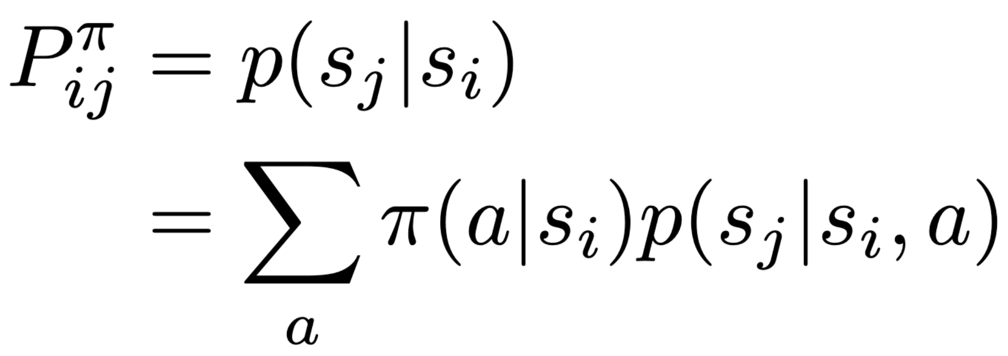
\begin{align*}
P^\pi_{ij} &= p(s_j|s_i) \\ &= \sum_{a}\pi(a|s_i)p(s_j|s_i,a)
\end{align*}
\begin{align*}
v_{\pi}(s) = \sum_a \pi(a|s) \Big(r(s,a) + \gamma \sum_{s'}p(s'|s,a) v_{\pi}(s')\Big)
\end{align*}

Bellman Equation in Matrix Form

The Bellman value equation, for a given , can be expressed using matrices,
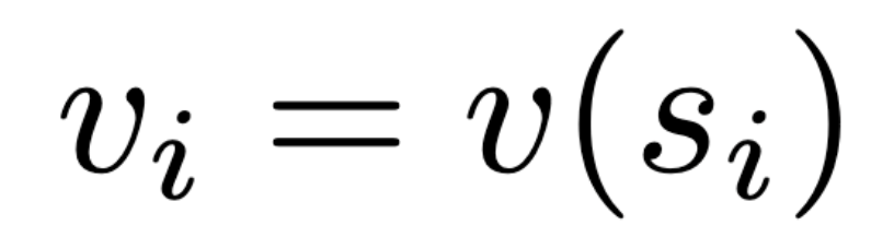
\[ \mathbf{v} = \mathbf{r}^\pi + \gamma\mathbf{P}^\pi\mathbf{v} \]

This is a linear equation that can be solved directly:
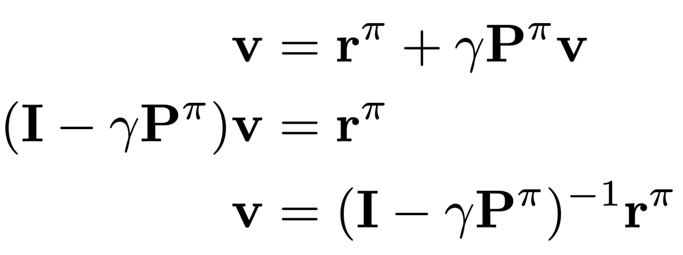
\begin{align*}
\mathbf{v} &= \mathbf{r}^\pi + \gamma\mathbf{P}^\pi\mathbf{v} \\ (\mathbf{I} - \gamma\mathbf{P}^\pi)\mathbf{v} &= \mathbf{r}^\pi \\ \mathbf{v} &= (\mathbf{I} - \gamma\mathbf{P}^\pi)^{-1}\mathbf{r}^\pi
\end{align*}

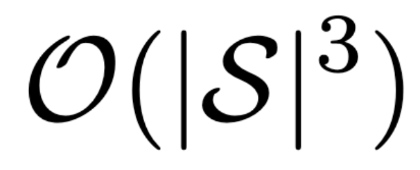
Computational complexity is

\begin{align*}
\mathcal{O}(|\mathcal{S}|^3)
\end{align*}

only possible for small problems

Iterative methods for larger problems

➢Dynamic programming

➢Monte-Carlo evaluation

➢Temporal-Difference learning

​

Solving the Bellman Optimality Equation

➢The Bellman optimality equation is non-linear

​

➢Cannot use the same direct matrix solution as for policy optimization (in general)

​

​

➢Many iterative solution methods:

​

➢Using models / dynamic programming

➢Value iteration

➢Policy iteration

​

➢Using samples

➢Monte Carlo

➢Q-learning

➢SARSA

Take home message

•Summary

•RL algorithms can be applied to environments that can be described as an MDP

•The goal of the RL agent is to learn a policy that maximizes the expected return

•Policies can be evaluated using value functions

•Bellman equations are recursive formulas for the value functions

•RL algorithms are heavily based on Bellman equations

​

Take home message