
Reinforcement Learning · Lecture 5

Model-Free Control
Rafael Fernandes Cunha

rafaelcunha2013.github.io

Today’s topics

1.Recap Monte Carlo and TD-learning

2.Model-Free Control

1.Monte Carlo

2.SARSA

3.Q-learning

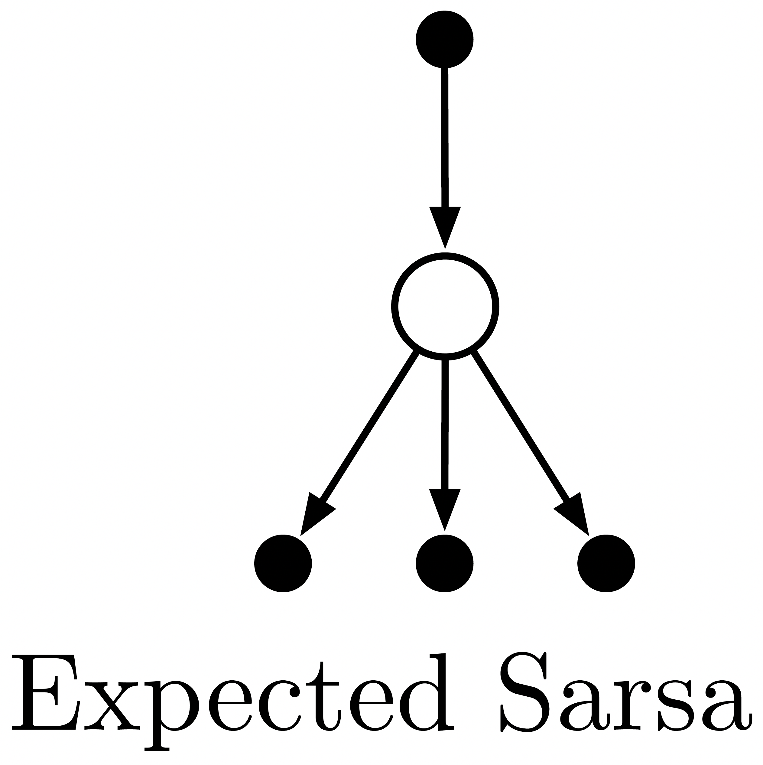
4.Expected SARSA

5.Double Q-learning

6.DQN

3.Importance Sampling

2

1.Explain the SARSA algorithm

2.Explain Q-learning

3.Compare On-policy x Off-policy algorithms

4.Illustrate the difference between Q-learning
and Double Q-learning

5.Explain the expected SARSA algorithm

6.Explain the intuition behind DQN

7.Summarize the importance Sampling
methodology.

Learning outcomes

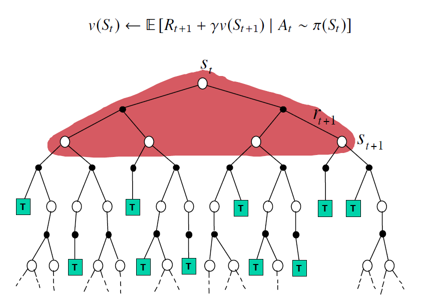
Dynamic Programming Backup

\begin{align*}
    v(S_t) \leftarrow \mathbb{E}[R_{t+1} + \gamma v(S_{t+1} | A_t \sim \pi(S_t))] 
\end{align*}
\begin{align*}
    v(s) \leftarrow \sum_a \pi(a|s)\sum_{s', r} p(s',r|s,a)(r+ \gamma v(s'))
\end{align*}

Expectation notation

Explicit probabilities

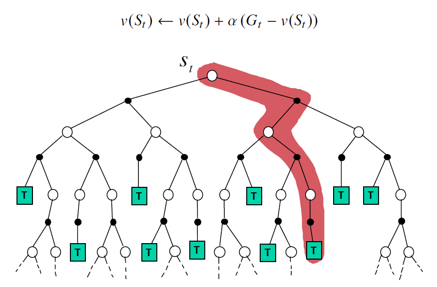
Monte-Carlo Backup
\begin{align*}
    v(S_t) \leftarrow v(S_t) + \alpha (G_t - v(S_t)) 
\end{align*}

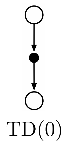
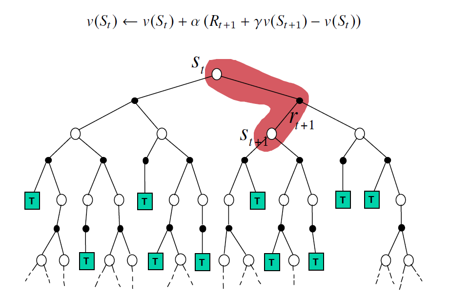
Temporal-Difference Learning Backup
\begin{align*}
    v(S_t) \leftarrow v(S_t) + \alpha (R_{t+1} + \gamma v(S_{t+1}) - v(S_t)) 
\end{align*}

Sampled Returns (MC) vs Bootstrapping (TD)

MC target (Sampled Returns):

TD target (Bootstrapping):

Biased. Uses next reward plus estimated value (bootstrapping).

High Variance - Return depends on many random actions, transitions, rewards.

Low Variance: TD target depends on one random action, transition, reward.

Variance:

Variance:

Bias:

\begin{align*}
    G_t = R_{t+1} + \gamma R_{t+2} + \cdots 
\end{align*}
\begin{align*}
    R_{t+1} + \gamma v_t(S_{t+1}) 
\end{align*}

Update:

Unbiased. Uses actual returns.

Bias:

Update:

Offline – It needs to wait until the end of the episode to compute the return.

Online – It can update after each step.

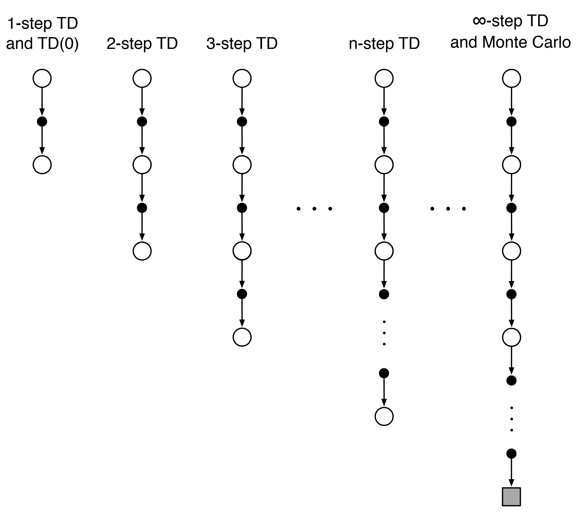
Between MC and TD: Multi-Step TD

Unified View of
Reinforcement Learning
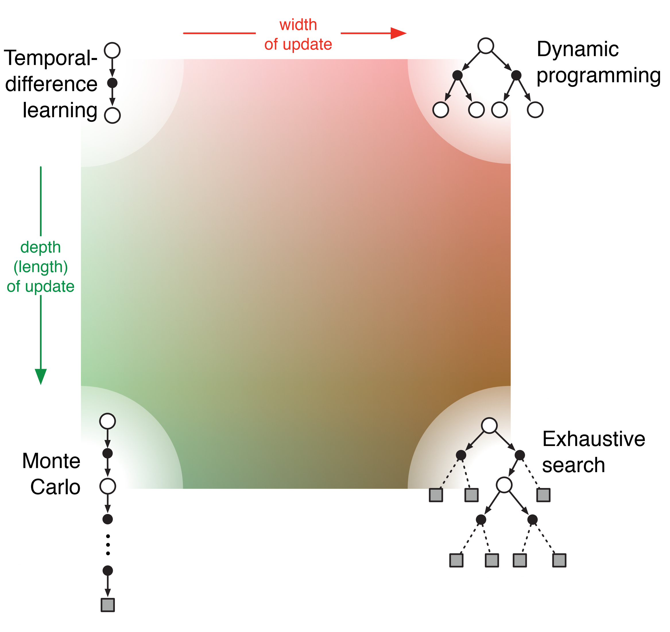
Multi-Step Prediction

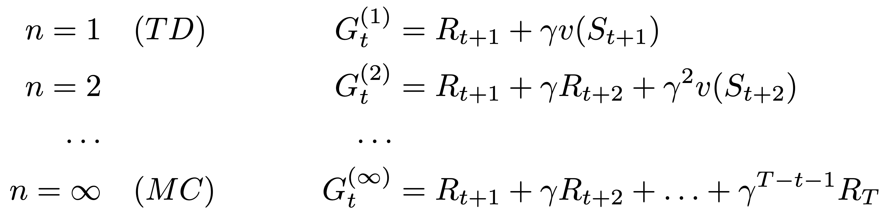
Let the TD target look
steps into the future
\begin{align*}
n &= 1 \quad (TD) & G_t^{(1)} &= R_{t+1} + \gamma v(S_{t+1}) \\ n &= 2 & G_t^{(2)} &= R_{t+1} + \gamma R_{t+2} + \gamma^2 v(S_{t+2}) \\ &\ldots & \ldots\; & \\ n &= \infty \quad (MC) & G_t^{(\infty)} &= R_{t+1} + \gamma R_{t+2} + \ldots + \gamma^{T-t-1} R_T
\end{align*}
\begin{align*}
n &= 1 \quad (TD) & G_t^{(1)} &= R_{t+1} + \gamma v(S_{t+1}) \\ n &= 2 & G_t^{(2)} &= R_{t+1} + \gamma R_{t+2} + \gamma^2 v(S_{t+2}) \\ &\ldots & \ldots\; & \\ n &= \infty \quad (MC) & G_t^{(\infty)} &= R_{t+1} + \gamma R_{t+2} + \ldots + \gamma^{T-t-1} R_T
\end{align*}
\begin{align*}
n &= 1 \quad (TD) & G_t^{(1)} &= R_{t+1} + \gamma v(S_{t+1}) \\ n &= 2 & G_t^{(2)} &= R_{t+1} + \gamma R_{t+2} + \gamma^2 v(S_{t+2}) \\ &\ldots & \ldots\; & \\ n &= \infty \quad (MC) & G_t^{(\infty)} &= R_{t+1} + \gamma R_{t+2} + \ldots + \gamma^{T-t-1} R_T
\end{align*}

-step returns

\begin{align*}
G^{(n)}_t \doteq R_{t+1} + \gamma R_{t+2} + \ldots + \gamma^{n-1} R_{t+n} + \gamma^n v(S_{t+n})
\end{align*}
\begin{align*}
n &= 1 \quad (TD) & G_t^{(1)} &= R_{t+1} + \gamma v(S_{t+1}) \\ n &= 2 & G_t^{(2)} &= R_{t+1} + \gamma R_{t+2} + \gamma^2 v(S_{t+2}) \\ &\ldots & \ldots\; & \\ n &= \infty \quad (MC) & G_t^{(\infty)} &= R_{t+1} + \gamma R_{t+2} + \ldots + \gamma^{T-t-1} R_T
\end{align*}
\begin{align*}
n &= 1 \quad (TD) & G_t^{(1)} &= R_{t+1} + \gamma v(S_{t+1}) \\ n &= 2 & G_t^{(2)} &= R_{t+1} + \gamma R_{t+2} + \gamma^2 v(S_{t+2}) \\ &\ldots & \ldots\; & \\ n &= \infty \quad (MC) & G_t^{(\infty)} &= R_{t+1} + \gamma R_{t+2} + \ldots + \gamma^{T-t-1} R_T
\end{align*}

n-step TD

\begin{align*}
v_{k+1}(S_t) \leftarrow v_k(S_t) + \alpha\Big(G^{(n)}_t - v_k(S_t)\Big)
\end{align*}

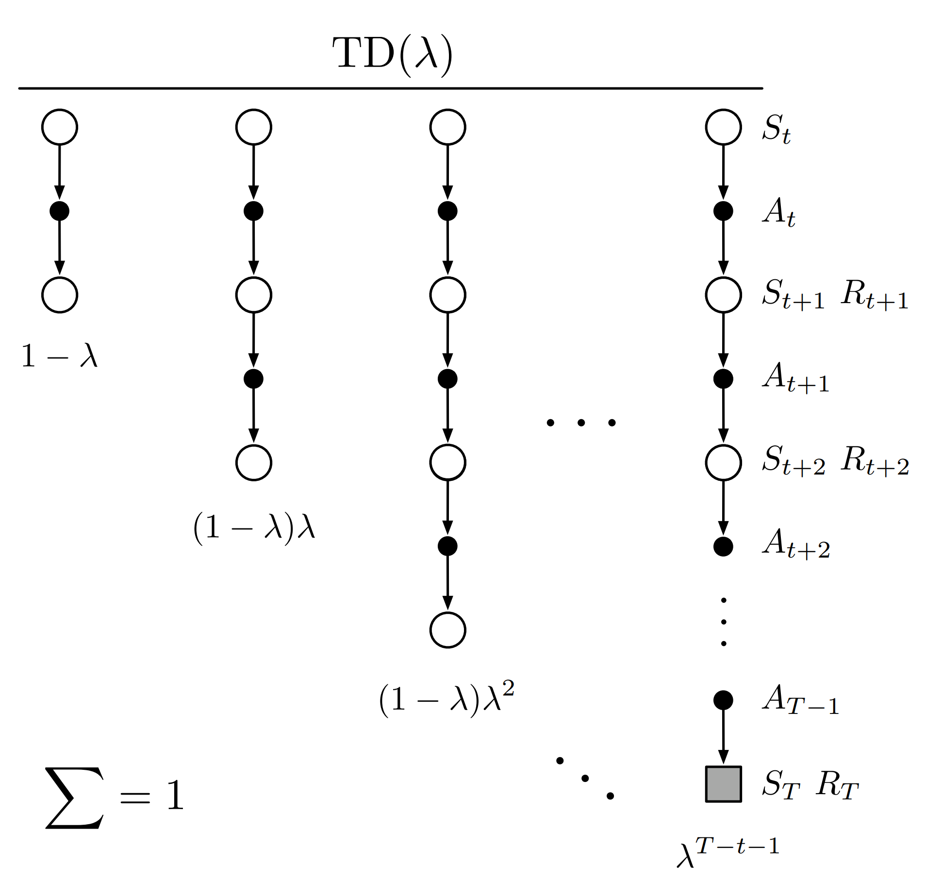
Mixed Multi-Step Returns

TD(0)

\begin{align*}
 G_t^{\lambda = 0} = R_{t+1} + \gamma v(S_{t+1}) 
\end{align*}

MC

\begin{align*}
G_t^{\lambda = 1} = R_{t+1} + \gamma G_{t+1}
\end{align*}

Mixed Multi-Step Returns

\begin{align*}
G^{(\lambda)}_t = R_{t+1} + \gamma\Big((1 - \lambda) v(S_{t+1}) + \lambda G^{(\lambda)}_{t+1}\Big)
\end{align*}

Incremental Update rule

NewEstimate

OldEstimate

StepSize

InformativeValue

Estimate

Target

OldEstimate

-

Prediction:

Each algorithm changes only the Target value!

Algorithms: Model-Free Prediction

Monte Carlo

TD(0)

n-step TD

TD(

Mixed Multi-Step Returns

\begin{align*}
G^{(\lambda)}_t = R_{t+1} + \gamma\Big((1 - \lambda) v(S_{t+1}) + \lambda G^{(\lambda)}_{t+1}\Big)
\end{align*}

-step returns

\begin{align*}
G^{(n)}_t \doteq R_{t+1} + \gamma R_{t+2} + \ldots + \gamma^{n-1} R_{t+n} + \gamma^n v(S_{t+n})
\end{align*}

Sampled Returns

Bootstrapping

Model-Free Control

➢Model-free prediction

➢Estimate the value function of an unknown MDP

➢Monte Carlo first/every visit

➢TD-learning (TD(0), n-step TD, TD())

➢Model-free control

➢Optimize the value function of an unknown MDP

➢Monte Carlo

➢SARSA

➢Q-learning

➢Expected SARSA

➢Double Q-learning

➢DQN

➢Importance Sampling

Today’s Lecture

Algorithms: Model-Free Control

Monte Carlo

SARSA

Q-learning

Expected SARSA

Double Q-learning

DQN

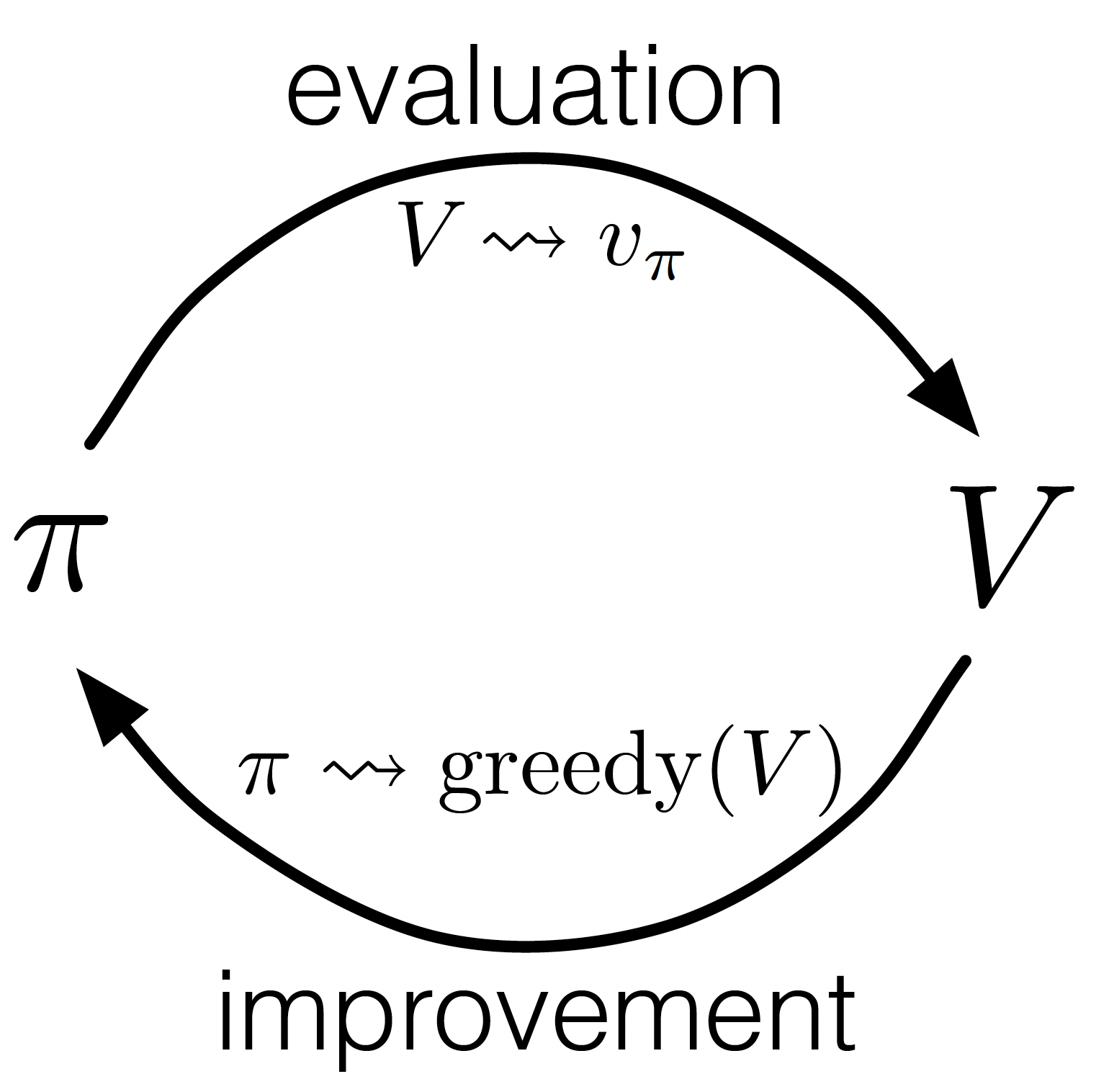
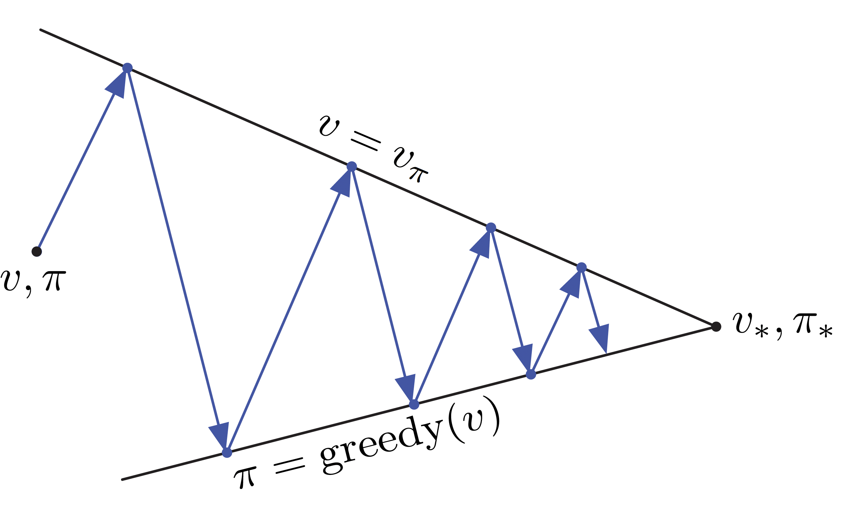
Generalized Policy Iteration (GPI)

Alternating with some chosen iterations.

Greedy policy improvement over
requires the model of the MDP

\begin{align*}
\pi'(s) = \underset{a}{\argmax}\sum_{s',r}p(s', r|s,a) \Big(r + \gamma  v_{\pi}(s')\Big)
\end{align*}

Greedy policy improvement over
is
model-free

\begin{align*}
\pi'(s) = \underset{a}{\argmax}q(s,a)
\end{align*}
\begin{align*}
(\mathcal{S}, \mathcal{A}, p, r, \gamma)
\end{align*}

Generalized Policy Iteration (GPI)

Alternating with some chosen iterations.

Policy evaluation: Monte-Carlo

Policy improvement: Greedy Policy?

What is the problem here?

Can’t sample all s, a, when
learning by interaction!

\begin{align*}
     \pi_0 \overset{\text{E}}{\longrightarrow} q_{\pi_0} \overset{\text{I}}{\longrightarrow}  \pi_1 \overset{\text{E}}{\longrightarrow} q_{\pi_1} \overset{\text{I}}{\longrightarrow}  \pi_2 \overset{\text{E}}{\longrightarrow} \cdots \overset{\text{I}}{\longrightarrow}  \pi_* \overset{\text{E}}{\longrightarrow} q_{\pi_*}  
\end{align*}

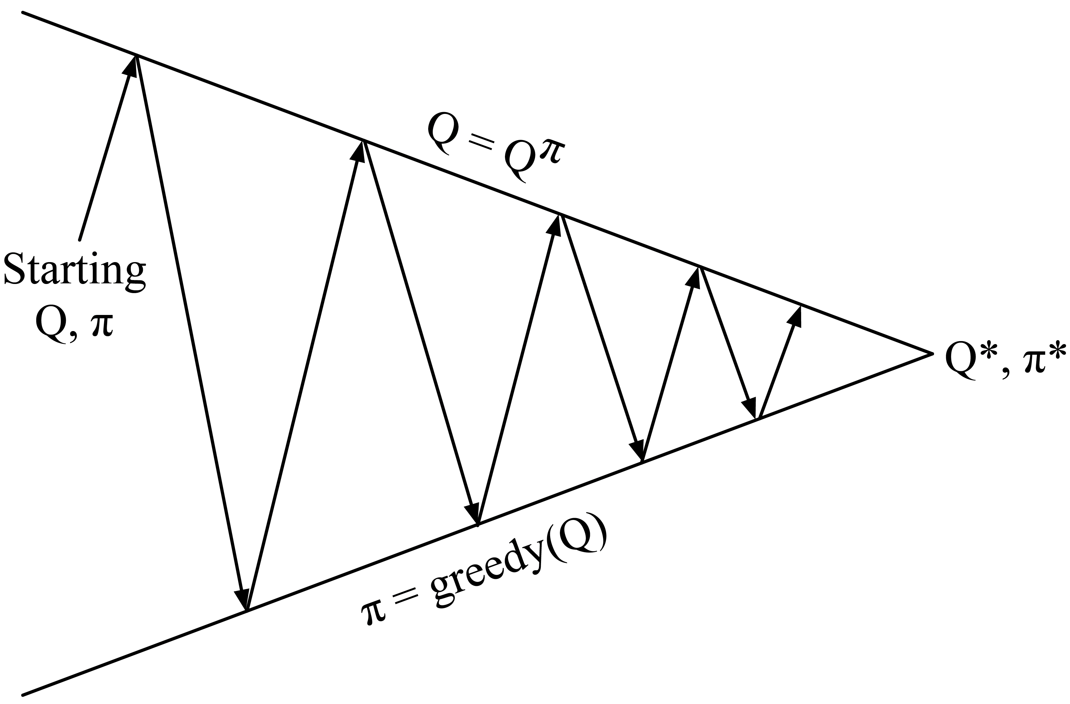
Generalized Policy Iteration (GPI)

Alternating with some chosen iterations.

Policy evaluation: Monte-Carlo

Policy improvement: -greedy Policy!

Keep exploring all s, a, when
learning by interaction!
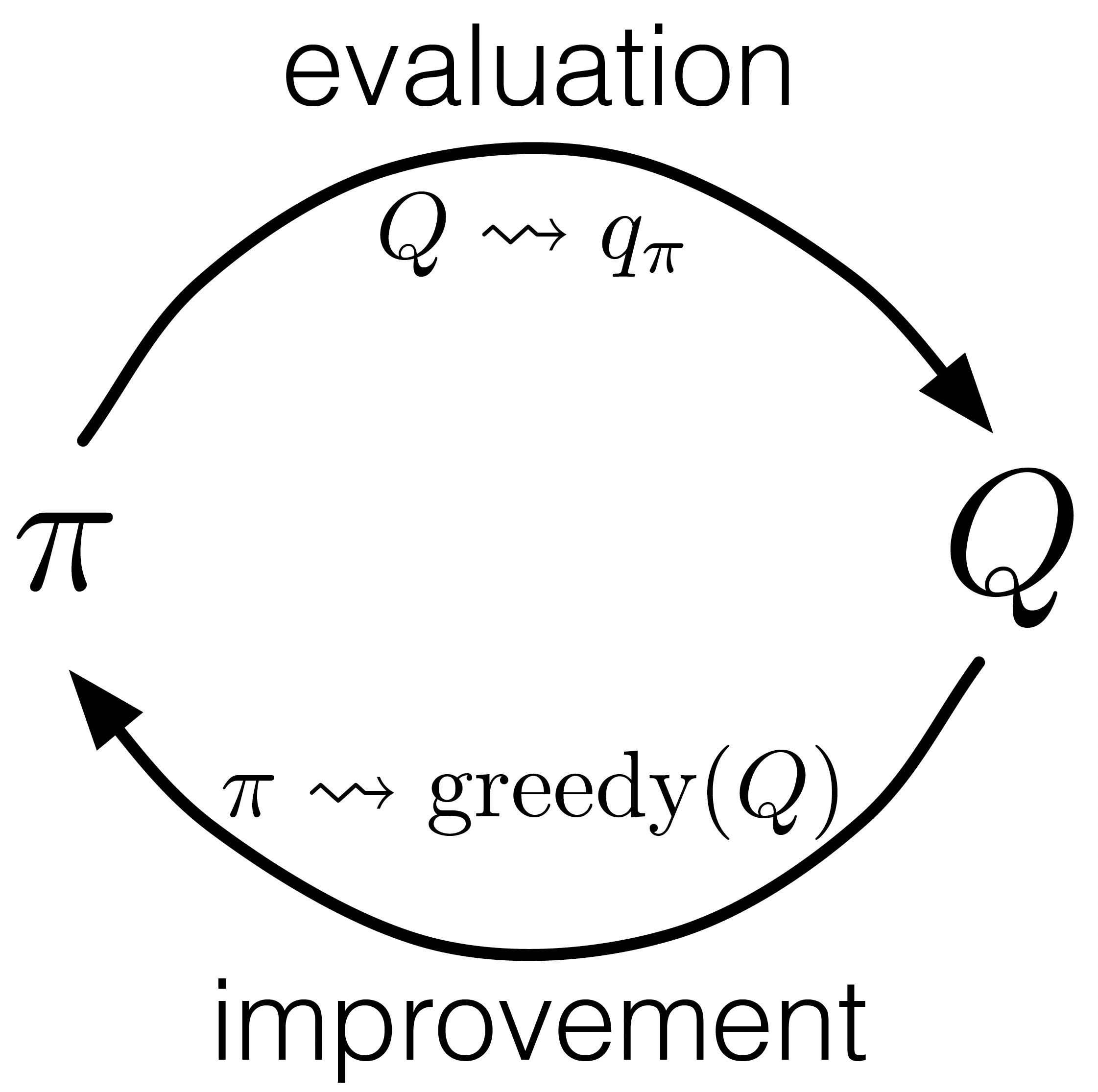
-greedy
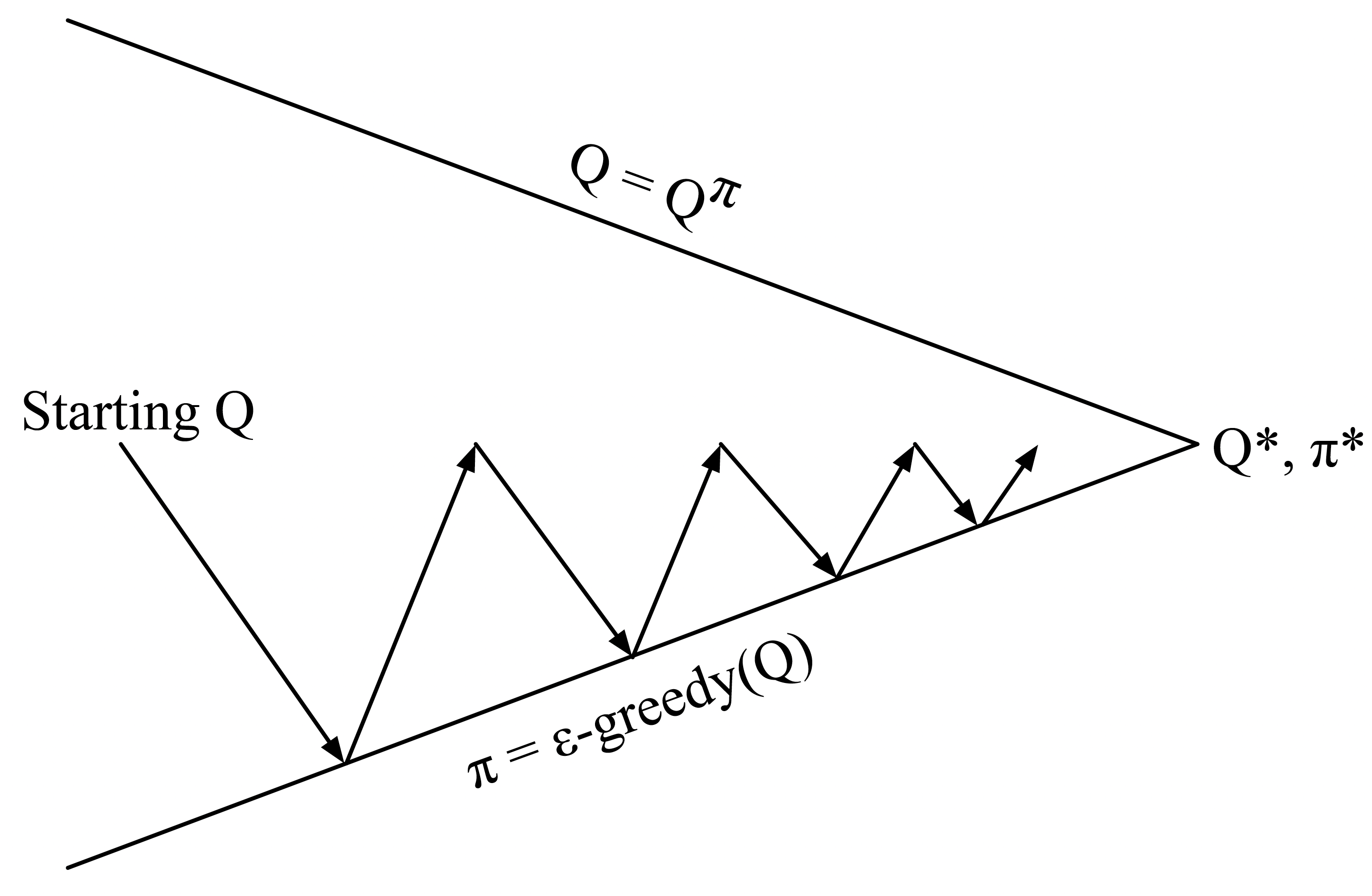
\begin{align*}
     \pi_0 \overset{\text{E}}{\longrightarrow} q_{\pi_0} \overset{\text{I}}{\longrightarrow}  \pi_1 \overset{\text{E}}{\longrightarrow} q_{\pi_1} \overset{\text{I}}{\longrightarrow}  \pi_2 \overset{\text{E}}{\longrightarrow} \cdots \overset{\text{I}}{\longrightarrow}  \pi_* \overset{\text{E}}{\longrightarrow} q_{\pi_*}  
\end{align*}

Model-free control (MC)

Sample episode using , , …,

Generalizes the -greedy
bandit algorithm

Repeat

For each state and action in the episode,

\begin{align*}
 q(S_t, A_t) \leftarrow q(S_t, A_t) + \alpha_t (G_t - q(S_t, A_t))
\end{align*}
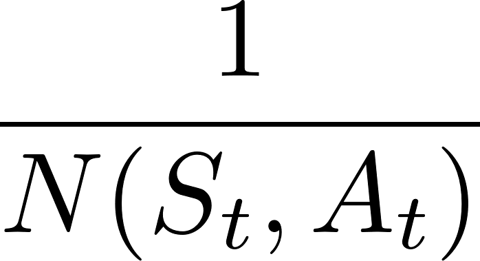
\begin{align*}
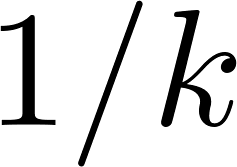
 \frac{1}{N(S_t, A_t)}
\end{align*}
\begin{align*}
1/k
\end{align*}

Improve policy based on new action-value function
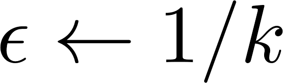
\begin{align*}
\epsilon \leftarrow 1/k
\end{align*}
\begin{align*}
\pi \leftarrow \epsilon\text{-greedy}(q)
\end{align*}

Algorithms: Model-Free Control

Monte Carlo

SARSA

Q-learning

Expected SARSA

Double Q-learning

DQN

\begin{align*}
    q(S_t, A_t) \leftarrow q(S_t, A_t) + \alpha \Big({\color{blue}G_t} - q(S_t, A_t)\Big) 
\end{align*}

GLIE

Greedy in the Limit with Infinite Exploration (GLIE)

All state-action pairs are explored infinitely many times

The policy converges to a greedy policy

Example

-greedy with

Theorem: GLIE Model-free control converges to the optimal action-value function,

\begin{align*}
\forall s, a \quad \lim_{t \rightarrow\infty} N_t(s,a) = \infty
\end{align*}
\begin{align*}
\lim_{t \rightarrow \infty} \pi_t(a|s) = \mathbb{I}(a = \argmax_{a' } q_t(s, a' ))
\end{align*}

Approach to ensure all actions are selected infinitely often

On-policy: Learn about target policy from experience sampled from behaviour policy

Off-policy: Learn about target policy from experience sampled from behaviour policy

➢Learn “counterfactually” about other things you could do: “what if …?”

➢“What if I would turn left” => new observations, rewards?

➢“What if I would play more defensively?” => different win probability?

➢“What if I would continue to go forward?” => how long until I bump into a wall?

➢“What if I would act greedy?” even if my behaviour policy is -greedy?

MC vs. TD Control

Temporal-difference (TD) learning has several advantages over Monte-Carlo (MC)

➢Lower variance

➢Online

➢Can learn from incomplete sequences

Let’s use TD instead of MC for control

➢Apply TD to

➢Use, e.g., -greedy policy improvement

➢Update every time-step

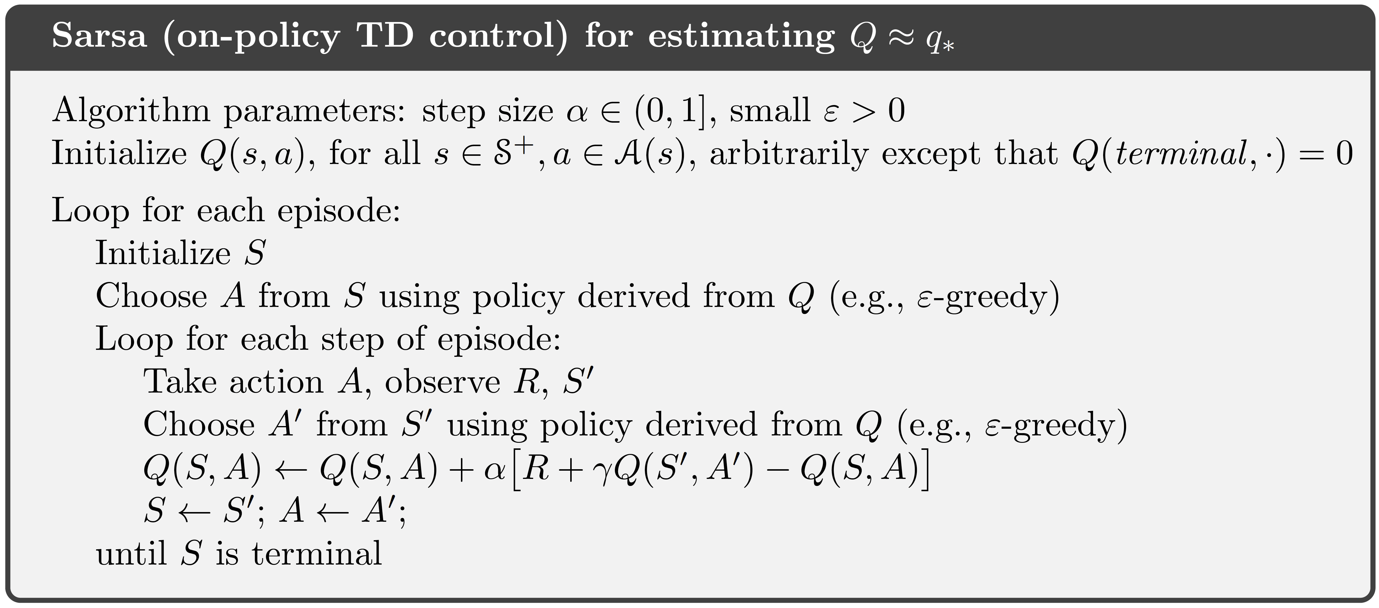
SARSA: On-policy TD Control

Policy evaluation: SARSA

Policy improvement: -greedy

Can I have another policy here?
Which condition should it obey?

Tabular SARSA converges to the optimal action-
value function,

Behaviour Policy is GLIE

Theorem

\begin{align*}
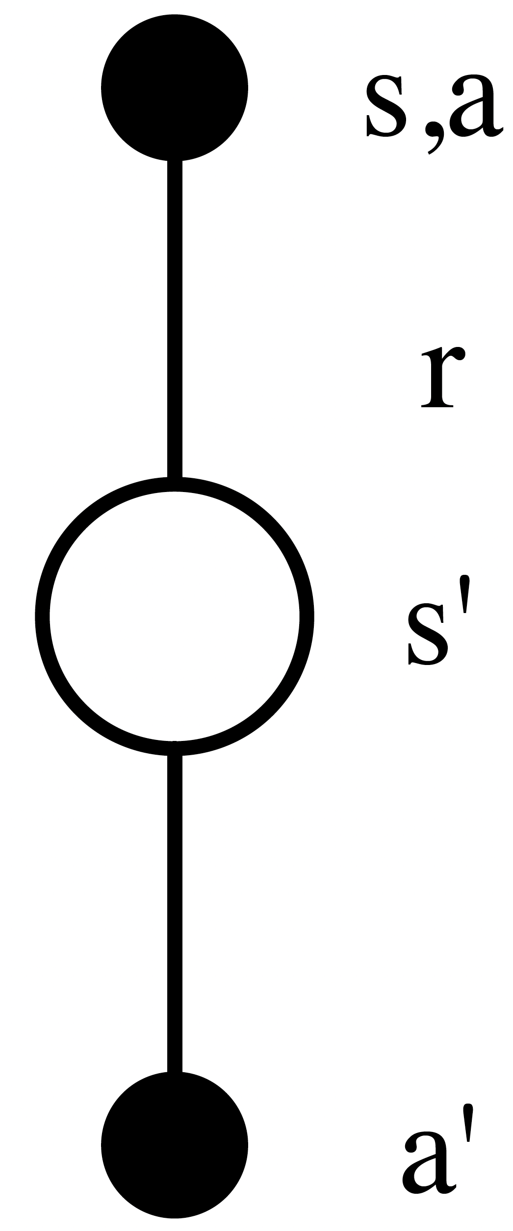
 q_{t+1}(S_t, A_t) = q_t(S_t, A_t) + \alpha_t (R_{t+1} + \gamma q_t(S_{t+1}, A_{t+1}) - q_t(S_t, A_t))
\end{align*}

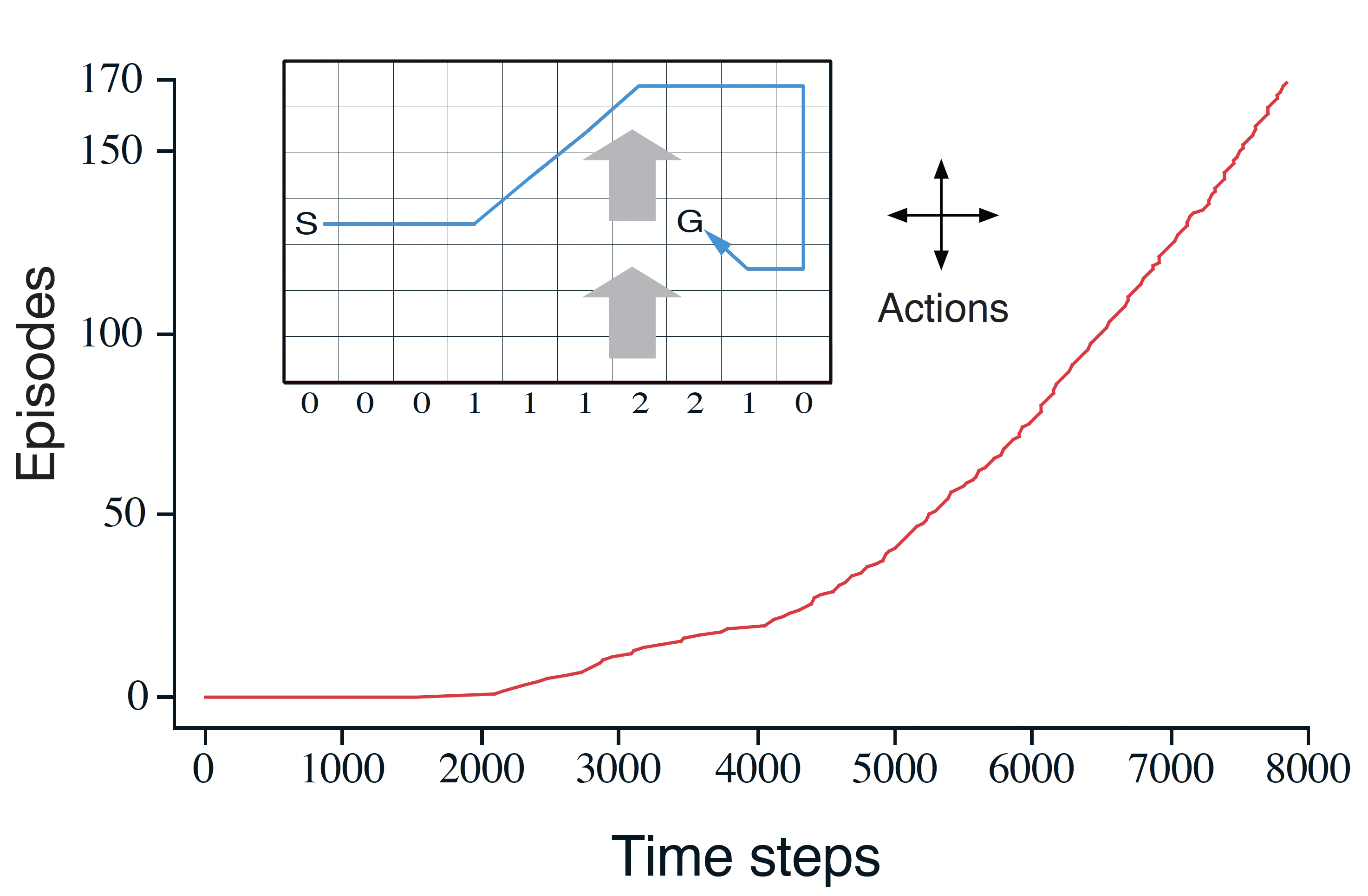
Example: Windy Gridworld

​

Policy: -greedy ()

Algorithm: SARSA ()

​

initial is 0 for all s, a

Why Monte-Carlo methods
cannot easily be used here?

Because termination is not
guaranteed for all policies.

Online learning methods
quickly learn a better policy

during the episode
.

Algorithms: Model-Free Control

Monte Carlo

SARSA

Q-learning

Expected SARSA

Double Q-learning

DQN

\begin{align*}
    q(S_t, A_t) \leftarrow q(S_t, A_t) + \alpha \Big({\color{blue}G_t} - q(S_t, A_t)\Big) 
\end{align*}
\begin{align*}
    q(S_t, A_t) \leftarrow q(S_t, A_t) + \alpha \Big({\color{blue}R_{t+1} + \gamma q(S_{t+1}, A_{t+1})} - q(S_t, A_t)\Big) 
\end{align*}

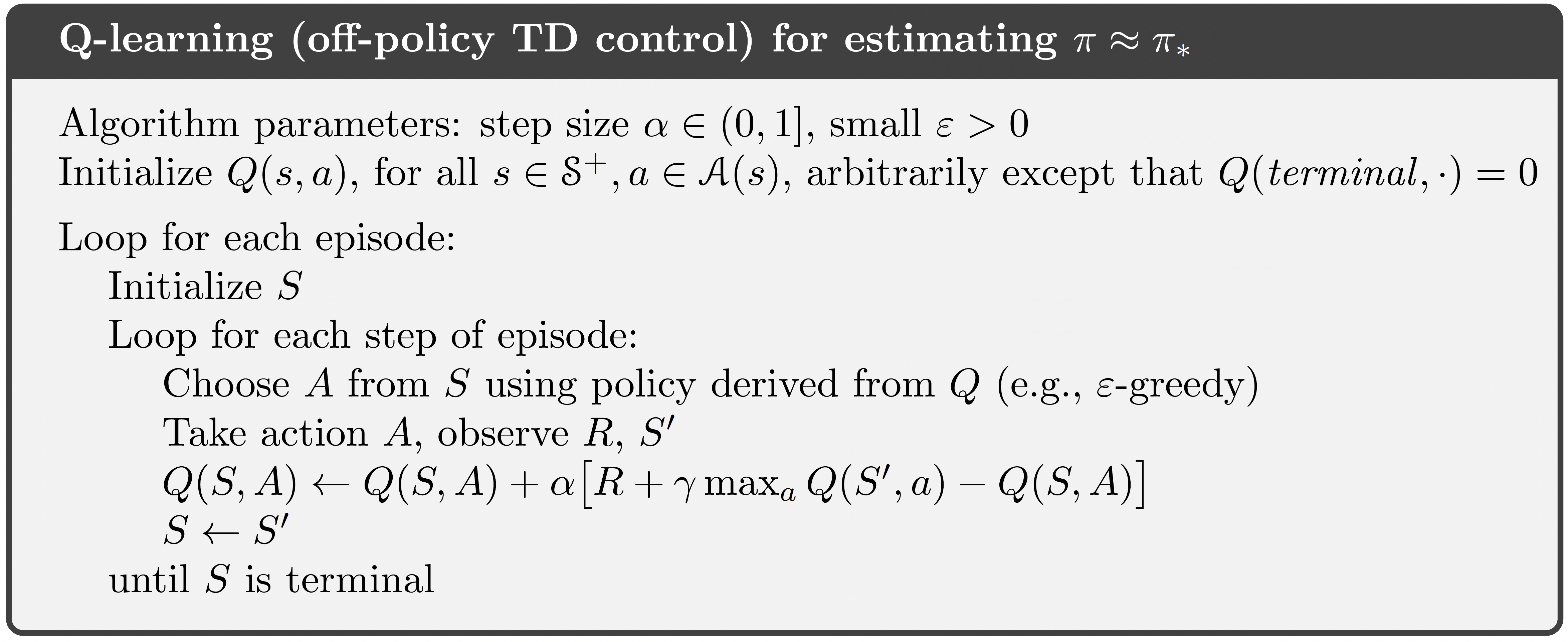
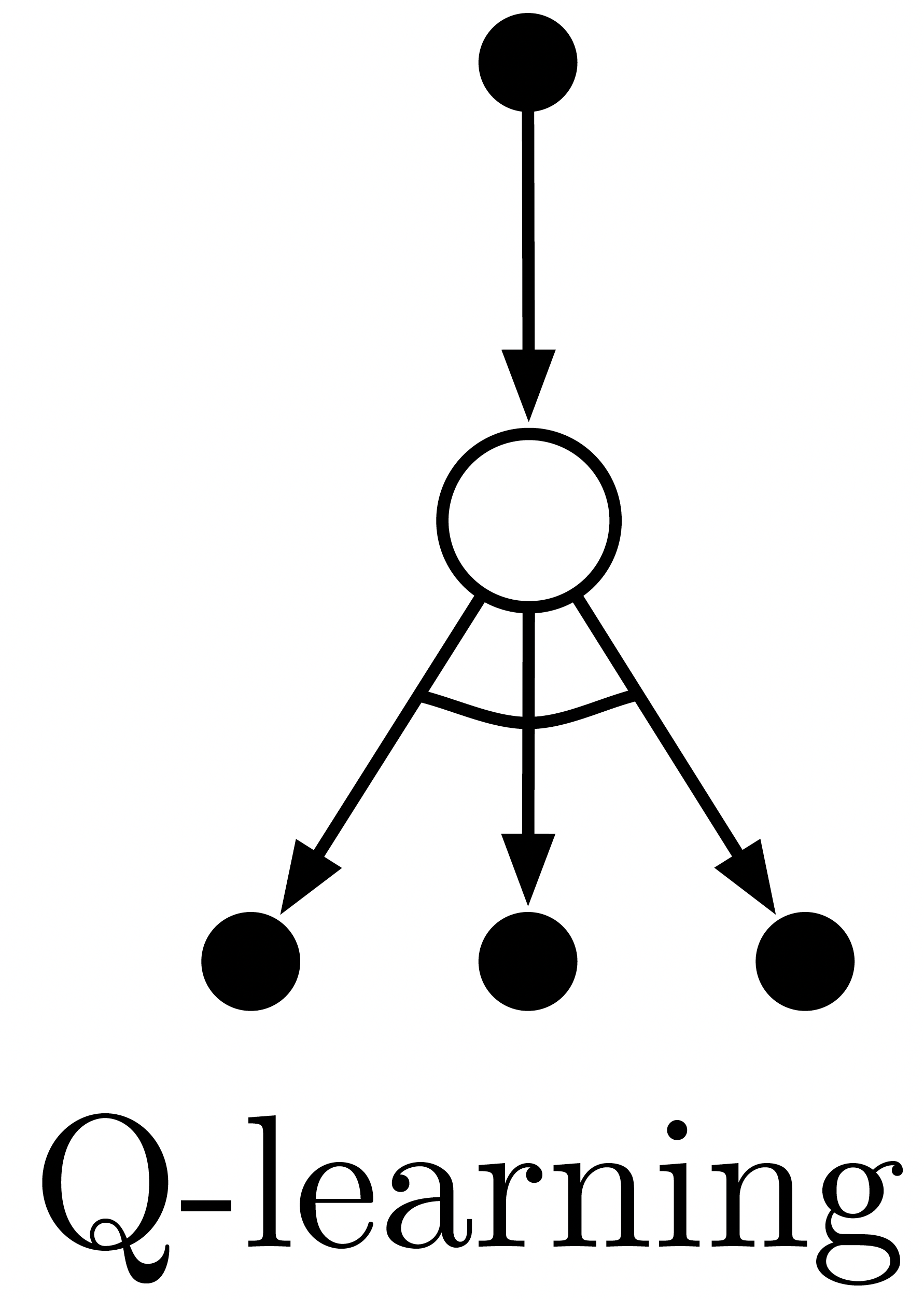
Q-learning (Off-policy Learning)

Evaluate target policy
to compute
or

Use behaviour policy to
generate actions

-greedy

greedy

\begin{align*}
  q_{t+1}(S_t, A_t) = q_t(S_t, A_t) + \alpha_t \Big(R_{t+1} + \gamma \max_{a'}  q_t(S_{t+1}, a' ) - q_t(S_t, A_t)\Big)
\end{align*}

Greedy policy does
not explore

➢Learn from observing humans or other agents (e.g., from logged data)

➢Re-use experience from old policies (e.g., from your own past experience)

➢Learn about multiple policies while following one policy

➢Learn about greedy policy while following exploratory policy

Q-learning Control Algorithm

Q-learning control converges to the optimal
action-value function,

Take each action in each state infinitely often

Theorem

From stochastic
approximation theory

Conditions required to
assure convergence
with probability 1

Note: no need for greedy behaviour!

Works for any policy that eventually
selects all actions sufficiently often!

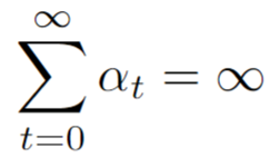
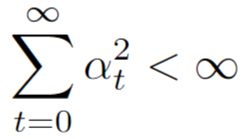
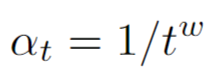
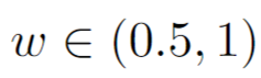
Recall the conditions over step-size of update rules

Steps are large enough to overcome any
initial conditions or random fluctuations

\begin{align*}
\sum_{t=0}^{\infty} \alpha_t = \infty
\end{align*}

Steps become small enough to
assure convergence

\begin{align*}
\sum_{t=0}^{\infty} \alpha_t^2 < \infty
\end{align*}
\begin{align*}
\alpha_t = 1/t^w
\end{align*}
\begin{align*}
w \in (0.5, 1)
\end{align*}
\begin{align*}
  q_{t+1}(S_t, A_t) = q_t(S_t, A_t) + \alpha_t \Big(R_{t+1} + \gamma \max_{a'}  q_t(S_{t+1}, a' ) - q_t(S_t, A_t)\Big)
\end{align*}

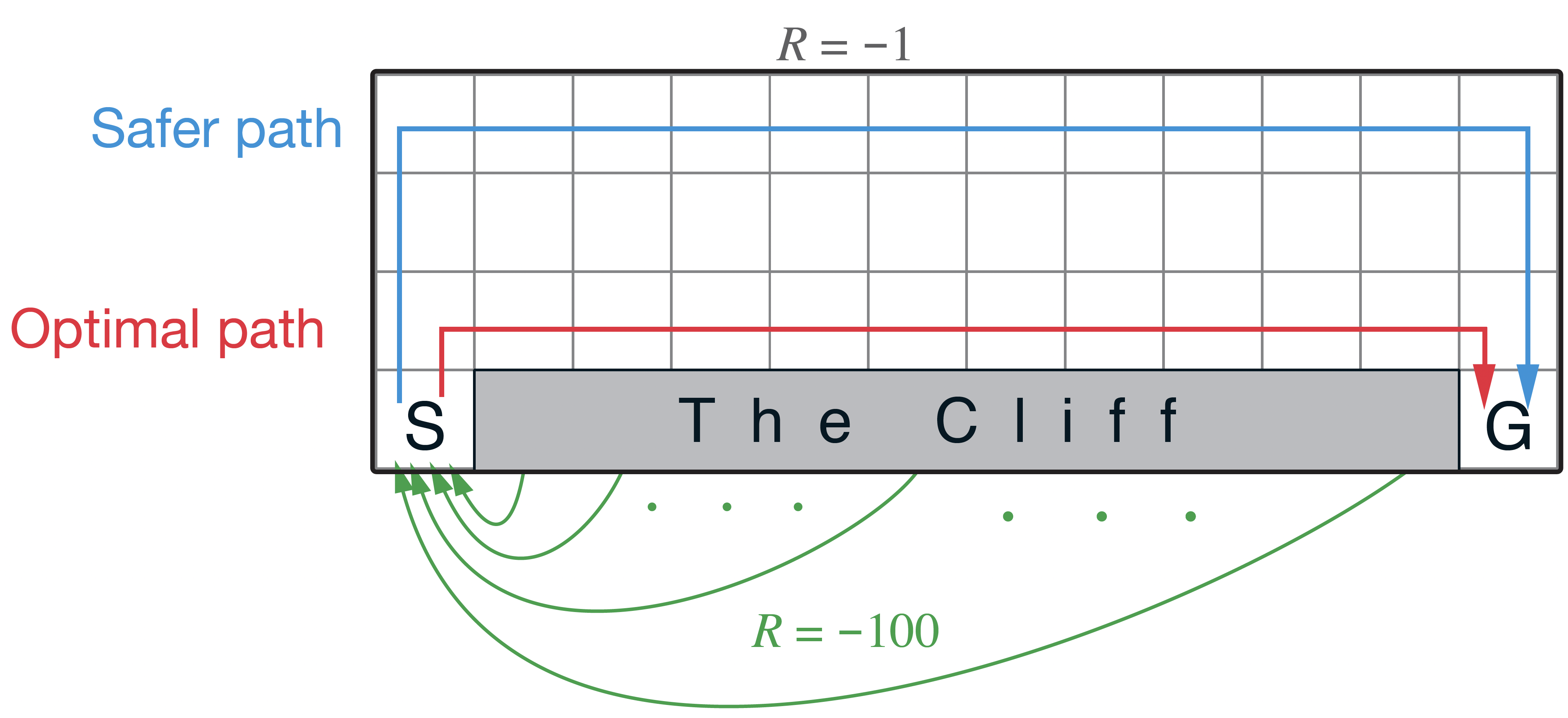
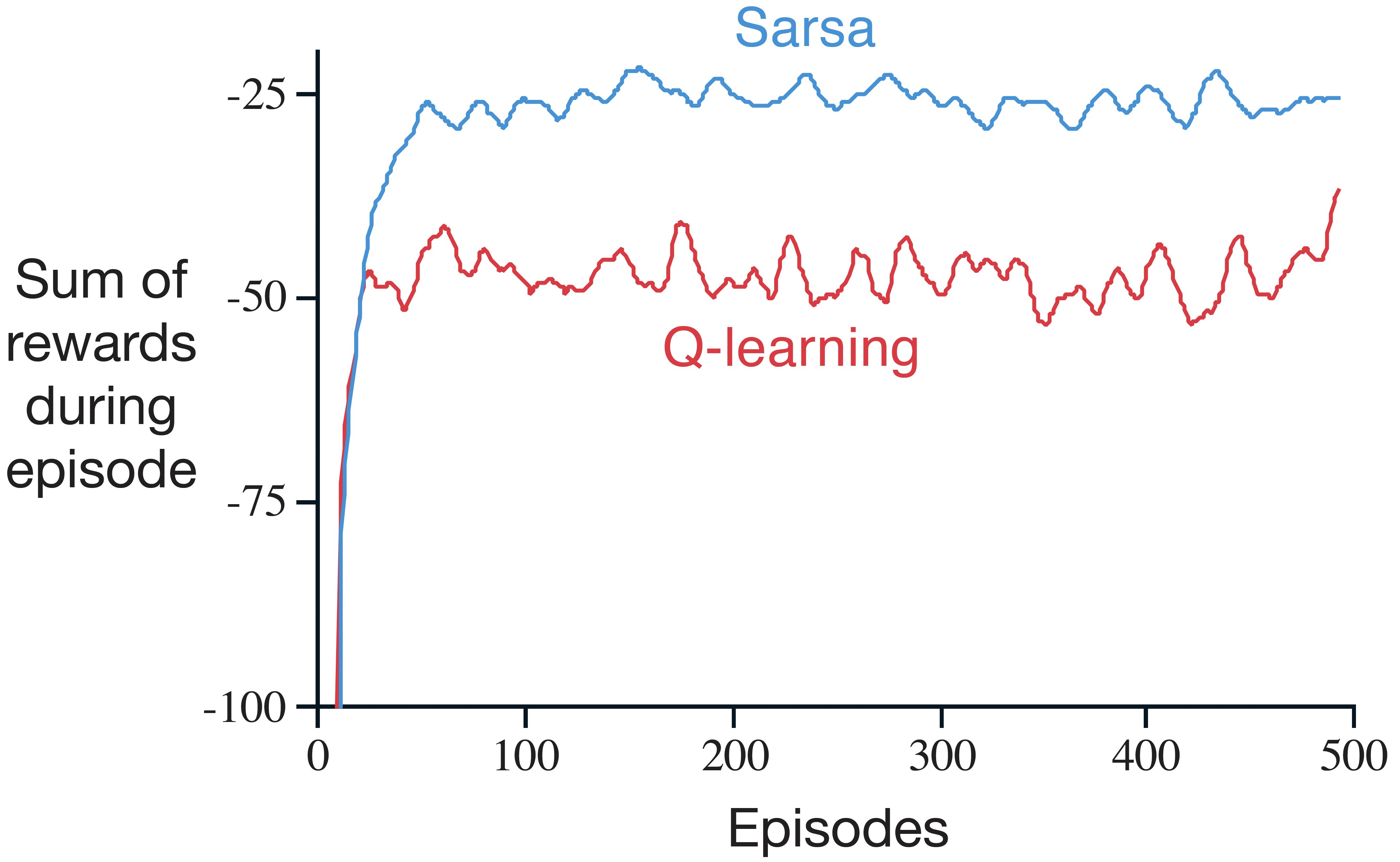
Example: Cliff Walking

SARSA (On-policy)

Q-learning (Off-policy)

Behaviour policy: -greedy

Target policy: -greedy

Behaviour policy: -greedy

Target policy: greedy

Example: Cliff Walking

SARSA (On-policy)

Q-learning (Off-policy)

Behaviour policy: -greedy

Target policy: -greedy

Behaviour policy: -greedy

Target policy: greedy

If , both methods would asymptotically converge to the optimal policy.

Which policy to evaluate when
running the experiment?

Algorithms: Model-Free Control

Monte Carlo

SARSA

Q-learning

Expected SARSA

Double Q-learning

DQN

\begin{align*}
    q(S_t, A_t) \leftarrow q(S_t, A_t) + \alpha \Big({\color{blue}G_t} - q(S_t, A_t)\Big) 
\end{align*}
\begin{align*}
    q(S_t, A_t) \leftarrow q(S_t, A_t) + \alpha \Big({\color{blue}R_{t+1} + \gamma q(S_{t+1}, A_{t+1})} - q(S_t, A_t)\Big) 
\end{align*}
\begin{align*}
       q(S_t, A_t) \leftarrow q(S_t, A_t) + \alpha \Big({\color{blue}R_{t+1} + \gamma 
 \max_{a'} q(S_{t+1}, a')} - q(S_t, A_t)\Big) 
\end{align*}

Expected SARSA

Expected SARSA (sometimes called “General Q-learning” )

Q-learning is a special case with greedy target policy

\begin{align*}
    q(S_t, A_t) \leftarrow q(S_t, A_t) + \alpha \Big(R_{t+1} + \gamma {\color{blue}\sum_{a'} \pi(a'|S_{t+1})} q(S_{t+1}, a') - q(S_t, A_t)\Big) 
\end{align*}

Consider probabilities
under

Update towards
value of alternative action

Action may be chosen using
behaviour
policy .

(off-policy learning)

Algorithms: Model-Free Control

Monte Carlo

SARSA

Q-learning

Expected SARSA

Double Q-learning

DQN

\begin{align*}
    q(S_t, A_t) \leftarrow q(S_t, A_t) + \alpha \Big({\color{blue}G_t} - q(S_t, A_t)\Big) 
\end{align*}
\begin{align*}
    q(S_t, A_t) \leftarrow q(S_t, A_t) + \alpha \Big({\color{blue}R_{t+1} + \gamma q(S_{t+1}, A_{t+1})} - q(S_t, A_t)\Big) 
\end{align*}
\begin{align*}
       q(S_t, A_t) \leftarrow q(S_t, A_t) + \alpha \Big({\color{blue}R_{t+1} + \gamma 
 \max_{a'} q(S_{t+1}, a')} - q(S_t, A_t)\Big) 
\end{align*}
\begin{align*}
    q(S_t, A_t) \leftarrow q(S_t, A_t) + \alpha \Big({\color{blue}R_{t+1} + \gamma \sum_{a'} \pi(a'|S_{t+1}) q(S_{t+1}, a')} - q(S_t, A_t)\Big) 
\end{align*}

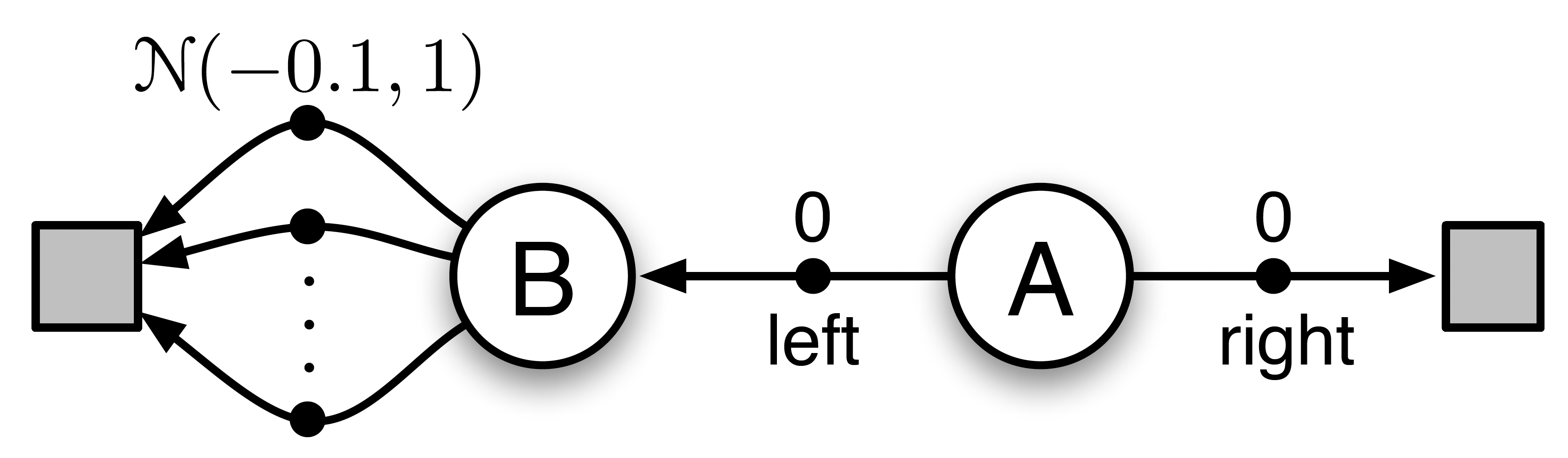
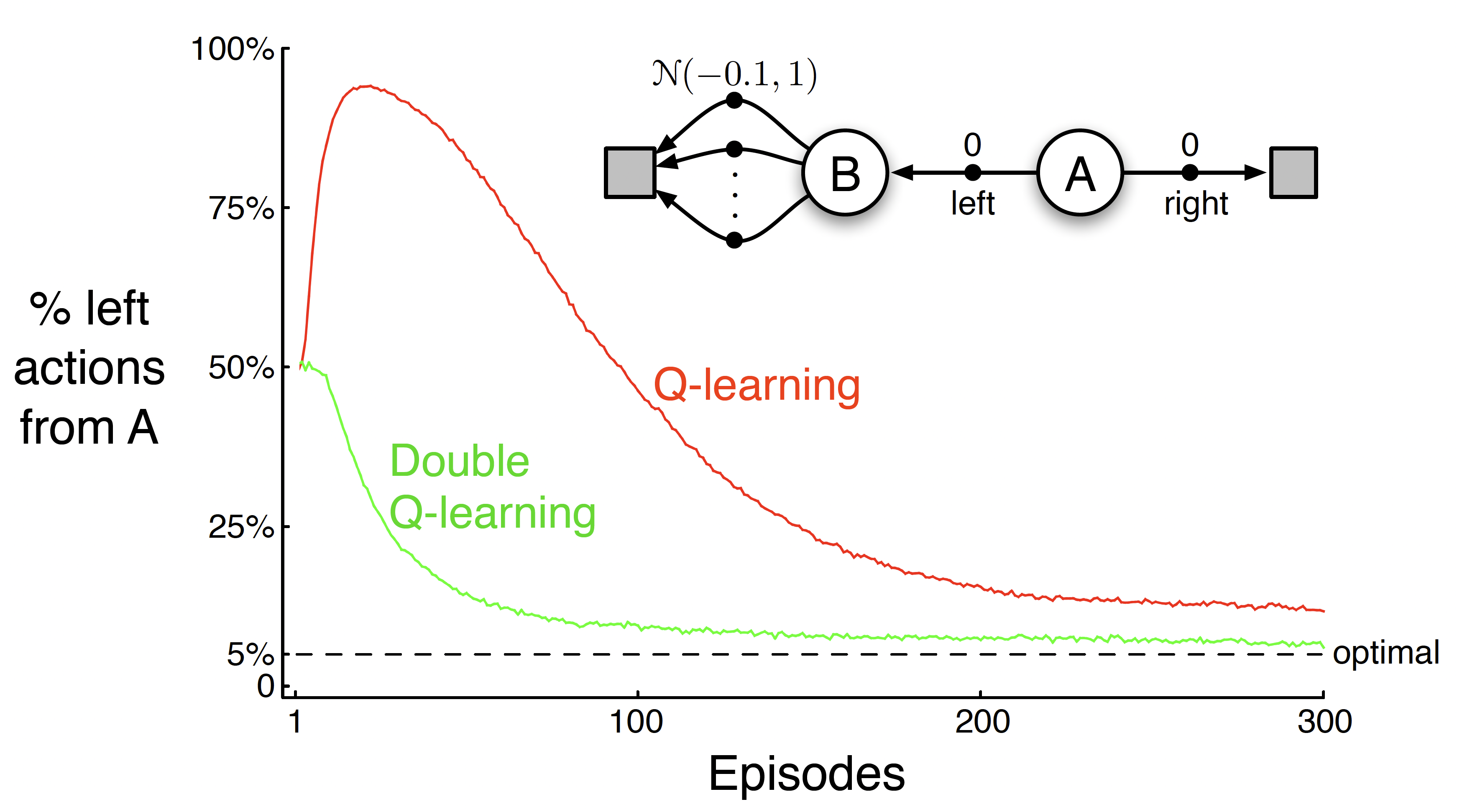
Example: Maximization Bias on Simple MDP

Policy: -greedy, with

% left actions from A

What is the optimal % of left actions
from A for this
-greedy policy ?

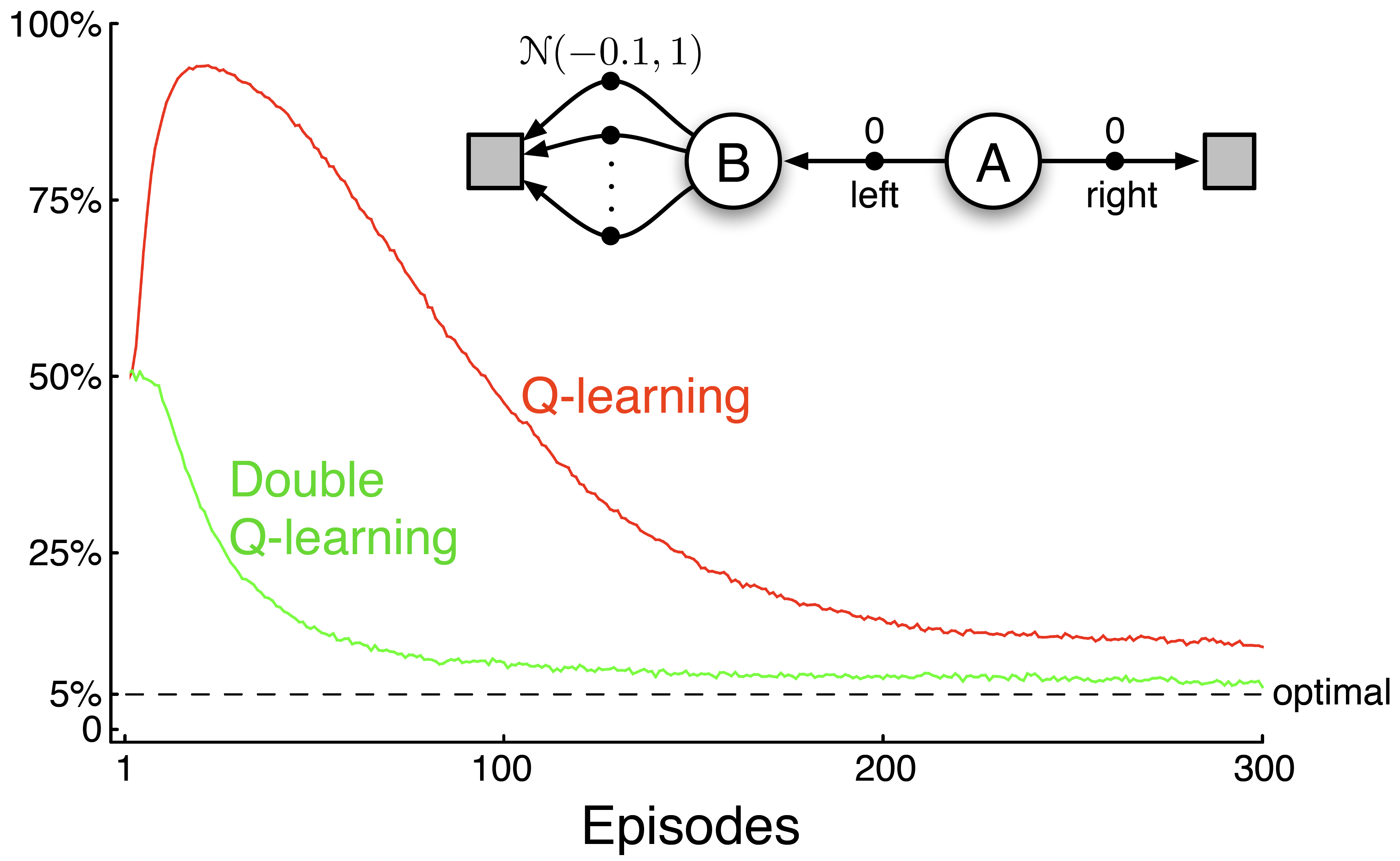
Example: Maximization Bias on Simple MDP

Policy: -greedy, with

% left actions from A

What is the optimal % of left actions
from A for this
-greedy policy ?

Example: Maximization Bias on Simple MDP

Policy: -greedy, with

% left actions from A

What is the optimal % of left actions
from A for this
-greedy policy ?

Why does q-learning initially selects
left actions from A with a high %?

\begin{align*}
    \max_{a'} q_t(S_{t+1}, a') = q_t \Big( S_{t+1}, \underset{a'}{\argmax} \; q_t(S_{t+1}, a') \Big)
\end{align*}

Q-learning overestimation

Selecting the action

Evaluating the action

Classical Q-learning has potential issues

But values are approximate

More likely to select overestimated values

Less likely to select underestimated values

This causes upward bias!

Same action-value function!

\begin{align*}
    \max_{a'} q_t(S_{t+1}, a') = q_t \Big( S_{t+1}, \underset{a'}{\argmax} \; q_t(S_{t+1}, a') \Big)
\end{align*}

Q-learning overestimation

Selecting the action

Evaluating the action

Q-learning overestimates because:

1) It uses the same action-value function to select and to evaluate the action!

2) It has the maximization term.

➢Q-learning will update if the state actually has high value

Decouple selection from evaluation

Solution

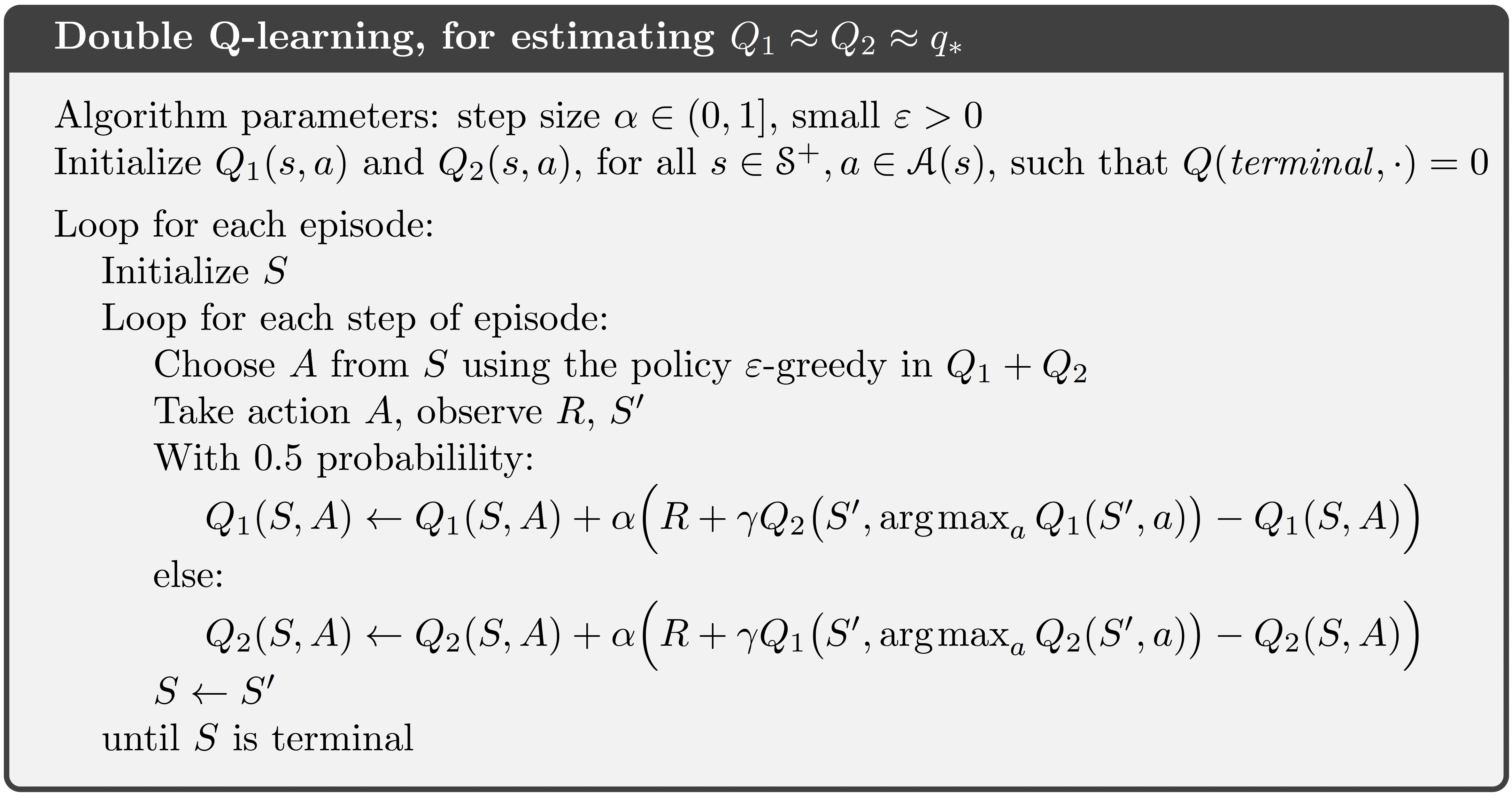
Double Q-learning

➢Store two action-value functions: and

➢Each , pick or (e.g., randomly) and update it.

​

➢Can use both to act (e.g., use policy based on )

Double Q-learning also converges to the optimal policy under the same conditions as Q-learning

\begin{align*}
    \textcolor{blue}{q_2}(S_t, A_t) \leftarrow \textcolor{blue}{q_2}(S_t, A_t) + \alpha \big[R_{t+1} + \gamma \textcolor{red}{q_1}\Big(S_{t+1}, \argmax_a \textcolor{blue}{q_2}(S_{t+1}, a)\Big) - \textcolor{blue}{q_2}(S_t, A_t)\Big] 
\end{align*}
\begin{align*}
        \textcolor{red}{q_1}(S_t, A_t) \leftarrow \textcolor{red}{q_1}(S_t, A_t) + \alpha \big[R_{t+1} + \gamma \textcolor{blue}{q_2}\Big(S_{t+1}, \argmax_a \textcolor{red}{q_1}(S_{t+1}, a)\Big) - \textcolor{red}{q_1}(S_t, A_t)\Big] 
\end{align*}

Example: Maximization Bias on Simple MDP

Double learning

The idea of double Q-learning can be generalized to other updates

Using -greedy in SARSA
can also overestimate

Solution

Double SARSA!

Algorithms: Model-Free Control

Monte Carlo

SARSA

Q-learning

Expected SARSA

Double Q-learning

DQN

\begin{align*}
    q(S_t, A_t) \leftarrow q(S_t, A_t) + \alpha \Big({\color{blue}G_t} - q(S_t, A_t)\Big) 
\end{align*}
\begin{align*}
    q(S_t, A_t) \leftarrow q(S_t, A_t) + \alpha \Big({\color{blue}R_{t+1} + \gamma q(S_{t+1}, A_{t+1})} - q(S_t, A_t)\Big) 
\end{align*}
\begin{align*}
       q(S_t, A_t) \leftarrow q(S_t, A_t) + \alpha \Big({\color{blue}R_{t+1} + \gamma 
 \max_{a'} q(S_{t+1}, a')} - q(S_t, A_t)\Big) 
\end{align*}
\begin{align*}
    q(S_t, A_t) \leftarrow q(S_t, A_t) + \alpha \Big({\color{blue}R_{t+1} + \gamma \sum_{a'} \pi(a'|S_{t+1}) q(S_{t+1}, a')} - q(S_t, A_t)\Big) 
\end{align*}
\begin{align*}
     \textcolor{blue}{q_2}(S_t, A_t) \leftarrow \textcolor{blue}{q_2}(S_t, A_t) + \alpha \big[R_{t+1} + \gamma \textcolor{red}{q_1}\Big(S_{t+1}, \argmax_a \textcolor{blue}{q_2}(S_{t+1}, a)\Big) - \textcolor{blue}{q_2}(S_t, A_t)\Big] 
\end{align*}
\begin{align*}
    \textcolor{red}{q_1}(S_t, A_t) \leftarrow \textcolor{red}{q_1}(S_t, A_t) + \alpha \big[R_{t+1} + \gamma \textcolor{blue}{q_2}\Big(S_{t+1}, \argmax_a \textcolor{red}{q_1}(S_{t+1}, a)\Big) - \textcolor{red}{q_1}(S_t, A_t)\Big] 
\end{align*}

Deep Reinforcement Learning

q-learning

Very big
state space

Impossible to
make a q-table

Approximate q-value
function by a neural network
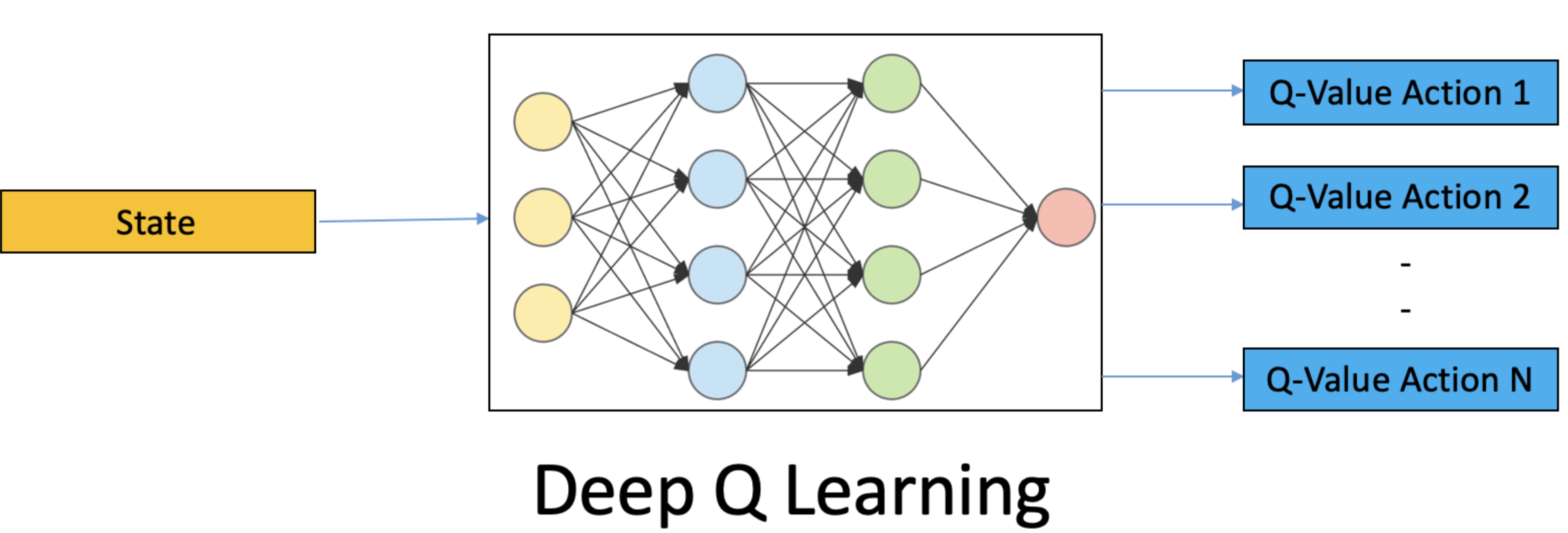
\begin{align*}
  q_{t+1}(S_t, A_t) = q_t(S_t, A_t) + \alpha_t \Big(R_{t+1} + \gamma \max_{a'}  q_t(S_{t+1}, a' ) - q_t(S_t, A_t)\Big)
\end{align*}

Weight update

\begin{align*}
       \Delta \mathbf{w} \propto \Big(R_{t+1} + \gamma \max_{a'} q_{\mathbf{w}}(S_{t+1}, a') - q_{\mathbf{w}}(S_t, A_t) \Big) \nabla_{\mathbf{w} }q_{\mathbf{w}}(S_t, A_t) 
\end{align*}

Deep Reinforcement Learning

q-learning

Very big
state space

Impossible to
make a q-table

Approximate q-value
function by a neural network

Simple Idea? Why did it take
so long to be invented?

\begin{align*}
  q_{t+1}(S_t, A_t) = q_t(S_t, A_t) + \alpha_t \Big(R_{t+1} + \gamma \max_{a'}  q_t(S_{t+1}, a' ) - q_t(S_t, A_t)\Big)
\end{align*}

Loss function

\begin{align*}
    L(\mathbf{w}) = \frac{1}{2} \Big(R_{t+1} + \gamma \Big[\!\!\Big[  \max_{a'} q_{\mathbf{w}}(S_{t+1}, a') \Big]\!\!\Big] - q_{\mathbf{w}}(S_t, A_t) \Big)^2 
\end{align*}

The deadly triad

•Bootstrapping

•Off-policy learning

•Function approximation

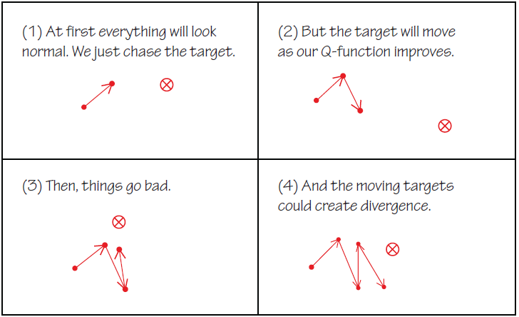
Make the algorithm diverge!

Learning data is not Independent and Identically distributed (iid)

Main difference when comparing with supervised learning datasets!

Experience Replay Buffer

Experience Replay Buffer store experiences (Transitions)

➢Sampling from this buffer helps get less correlated data.
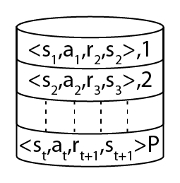
​

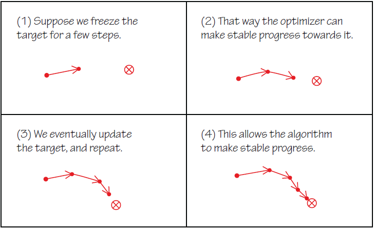
Target Network

Freeze Target network

Avoid chasing a moving target

Algorithms: Model-Free Control

Monte Carlo

SARSA

Q-learning

Expected SARSA

Double Q-learning

DQN

\begin{align*}
    q(S_t, A_t) \leftarrow q(S_t, A_t) + \alpha \Big({\color{blue}G_t} - q(S_t, A_t)\Big) 
\end{align*}
\begin{align*}
    q(S_t, A_t) \leftarrow q(S_t, A_t) + \alpha \Big({\color{blue}R_{t+1} + \gamma q(S_{t+1}, A_{t+1})} - q(S_t, A_t)\Big) 
\end{align*}
\begin{align*}
       q(S_t, A_t) \leftarrow q(S_t, A_t) + \alpha \Big({\color{blue}R_{t+1} + \gamma 
 \max_{a'} q(S_{t+1}, a')} - q(S_t, A_t)\Big) 
\end{align*}
\begin{align*}
    q(S_t, A_t) \leftarrow q(S_t, A_t) + \alpha \Big({\color{blue}R_{t+1} + \gamma \sum_{a'} \pi(a'|S_{t+1}) q(S_{t+1}, a')} - q(S_t, A_t)\Big) 
\end{align*}
\begin{align*}
     \textcolor{blue}{q_2}(S_t, A_t) \leftarrow \textcolor{blue}{q_2}(S_t, A_t) + \alpha \big[R_{t+1} + \gamma \textcolor{red}{q_1}\Big(S_{t+1}, \argmax_a \textcolor{blue}{q_2}(S_{t+1}, a)\Big) - \textcolor{blue}{q_2}(S_t, A_t)\Big] 
\end{align*}
\begin{align*}
    \textcolor{red}{q_1}(S_t, A_t) \leftarrow \textcolor{red}{q_1}(S_t, A_t) + \alpha \big[R_{t+1} + \gamma \textcolor{blue}{q_2}\Big(S_{t+1}, \argmax_a \textcolor{red}{q_1}(S_{t+1}, a)\Big) - \textcolor{red}{q_1}(S_t, A_t)\Big] 
\end{align*}
\begin{align*}
       \Delta \mathbf{w} \propto \Big(R_{t+1} + \gamma \max_{a'} q_{\mathbf{w}}(S_{t+1}, a') - q_{\mathbf{w}}(S_t, A_t) \Big) \nabla_{\mathbf{w} }q_{\mathbf{w}}(S_t, A_t) 
\end{align*}
\begin{align*}
    L(\mathbf{w}) = \frac{1}{2} \Big(R_{t+1} + \gamma \Big[\!\!\Big[  \max_{a'} q_{\mathbf{w}}(S_{t+1}, a') \Big]\!\!\Big] - q_{\mathbf{w}}(S_t, A_t) \Big)^2 
\end{align*}

Off-Policy Learning: Importance Sampling Corrections

Off-policy: Learn about target policy from experience sampled from behaviour policy

Evaluate target policy
to compute
or

Use behaviour policy
to generate actions

➢Q-learning is one example, but there are other options.

​

➢Note that you are sampling from one probability distribution to learn about a different one.

​

➢There are general tools to help with this.

​

➢Caveat: you can’t expect to learn about things you never do!

​

This may create problems!

Importance Sampling corrections

Given with random inputs ,
and distribution

Estimate the expectation of under
a different (target) distribution

Problem

Solution

Weigh the data by the ration

Intuition:

➢Scale up events that are rare under , but common under

➢Scale down events that are common under , but rare under

\begin{align*}
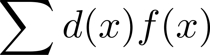
    \mathbb{E}_{x \sim d}[f(x)] =  
\end{align*}
\begin{align*}
    \sum d(x)f(x)  
\end{align*}
\begin{align*}
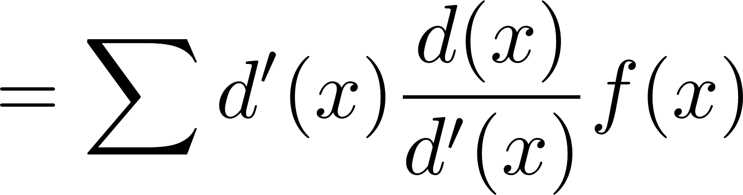
    = \sum d'(x) \frac{d(x)}{d' (x)}f(x) 
\end{align*}
\begin{align*}
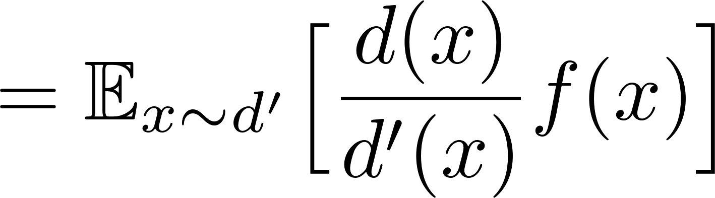
     =\mathbb{E}_{x \sim d' } \Big[ \frac{d(x)}{d' (x)} f(x) \Big] 
\end{align*}

Importance sampling corrections

➢Example: estimate one-step reward

➢Behaviour is
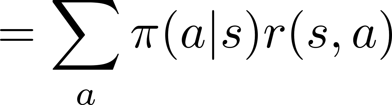
\begin{align*}
       = \sum_a \pi(a|s) r(s,a)  
\end{align*}
\begin{align*}
  = \sum \mu(a|s) \frac{\pi(a|s)}{\mu(a|s)}r(s,a)
\end{align*}
\begin{align*}
   = \mathbb{E} \Big[\frac{\pi(A_t|S_t)}{\mu(A_t|S_t)}R_{t+1} | S_t = s, A_t \sim \mu \Big] 
\end{align*}
\begin{align*}
        \mathbb{E}[R_{t+1}|S_t = s, A_t \sim \pi] 
\end{align*}

Importance sampling corrections

➢Example: estimate one-step reward

➢Behaviour is
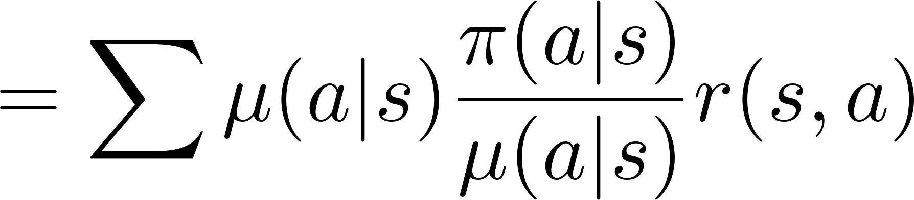
\begin{align*}
        \mathbb{E}[R_{t+1}|S_t = s, A_t \sim \pi] 
\end{align*}
\begin{align*}
   = \mathbb{E} \Big[\frac{\pi(A_t|S_t)}{\mu(A_t|S_t)}R_{t+1} | S_t = s, A_t \sim \mu \Big] 
\end{align*}
\begin{align*}
   = \mathbb{E} \Big[\frac{\pi(A_t|S_t)}{\mu(A_t|S_t)}R_{t+1} | S_t = s, A_t \sim \mu \Big] 
\end{align*}

Importance sampling corrections

➢Example: estimate one-step reward

➢Behaviour is

When following policy , use as unbiased sample!
\begin{align*}
        \mathbb{E}[R_{t+1}|S_t = s, A_t \sim \pi] 
\end{align*}
\begin{align*}
p_\pi(\tau) &= p_\pi(s_0, a_0, r_1, s_1, a_1, r_2, s_2) \\[1em] &= p_\pi(s_0, a_0, r_1, s_1, a_1) p(s_2, r_2 | s_0, a_0, r_1, s_1, a_1) \\[1em] &= p_\pi(s_0, a_0, r_1, s_1, a_1) p(s_2, r_2 | s_1, a_1) \\[1em] &= p_\pi(s_0, a_0, r_1, s_1) p_\pi(a_1 | s_0, a_0, r_1, s_1) p(s_2, r_2 | s_1, a_1) \\[1em] &= p_\pi(s_0, a_0, r_1, s_1) \pi(a_1 | s_1) p(s_2, r_2 | s_1, a_1) \\[1em] &= p_\pi(s_0, a_0) p(s_1, r_1 | s_0, a_0) \pi(a_1 | s_1) p(s_2, r_2 | s_1, a_1) \\[1em] &= p_\pi(s_0) \pi(a_0 | s_0) p(s_1, r_1 | s_0, a_0) \pi(a_1 | s_1) p(s_2, r_2 | s_1, a_1) \\[1em] &= p(s_0) \prod_{t=0}^{T-1} \pi(a_t | s_t) p(s_{t+1}, r_{t+1} | s_t, a_t)
\end{align*}
\begin{align*}
p_\pi(\tau) &= p_\pi(s_0, a_0, r_1, s_1, a_1, r_2, s_2) \\[1em] &= p_\pi(s_0, a_0, r_1, s_1, a_1) p(s_2, r_2 | s_0, a_0, r_1, s_1, a_1) \\[1em] &= p_\pi(s_0, a_0, r_1, s_1, a_1) p(s_2, r_2 | s_1, a_1) \\[1em] &= p_\pi(s_0, a_0, r_1, s_1) p_\pi(a_1 | s_0, a_0, r_1, s_1) p(s_2, r_2 | s_1, a_1) \\[1em] &= p_\pi(s_0, a_0, r_1, s_1) \pi(a_1 | s_1) p(s_2, r_2 | s_1, a_1) \\[1em] &= p_\pi(s_0, a_0) p(s_1, r_1 | s_0, a_0) \pi(a_1 | s_1) p(s_2, r_2 | s_1, a_1) \\[1em] &= p_\pi(s_0) \pi(a_0 | s_0) p(s_1, r_1 | s_0, a_0) \pi(a_1 | s_1) p(s_2, r_2 | s_1, a_1) \\[1em] &= p(s_0) \prod_{t=0}^{T-1} \pi(a_t | s_t) p(s_{t+1}, r_{t+1} | s_t, a_t)
\end{align*}
\begin{align*}
p_\pi(\tau) &= p_\pi(s_0, a_0, r_1, s_1, a_1, r_2, s_2) \\[1em] &= p_\pi(s_0, a_0, r_1, s_1, a_1) p(s_2, r_2 | s_0, a_0, r_1, s_1, a_1) \\[1em] &= p_\pi(s_0, a_0, r_1, s_1, a_1) p(s_2, r_2 | s_1, a_1) \\[1em] &= p_\pi(s_0, a_0, r_1, s_1) p_\pi(a_1 | s_0, a_0, r_1, s_1) p(s_2, r_2 | s_1, a_1) \\[1em] &= p_\pi(s_0, a_0, r_1, s_1) \pi(a_1 | s_1) p(s_2, r_2 | s_1, a_1) \\[1em] &= p_\pi(s_0, a_0) p(s_1, r_1 | s_0, a_0) \pi(a_1 | s_1) p(s_2, r_2 | s_1, a_1) \\[1em] &= p_\pi(s_0) \pi(a_0 | s_0) p(s_1, r_1 | s_0, a_0) \pi(a_1 | s_1) p(s_2, r_2 | s_1, a_1) \\[1em] &= p(s_0) \prod_{t=0}^{T-1} \pi(a_t | s_t) p(s_{t+1}, r_{t+1} | s_t, a_t)
\end{align*}

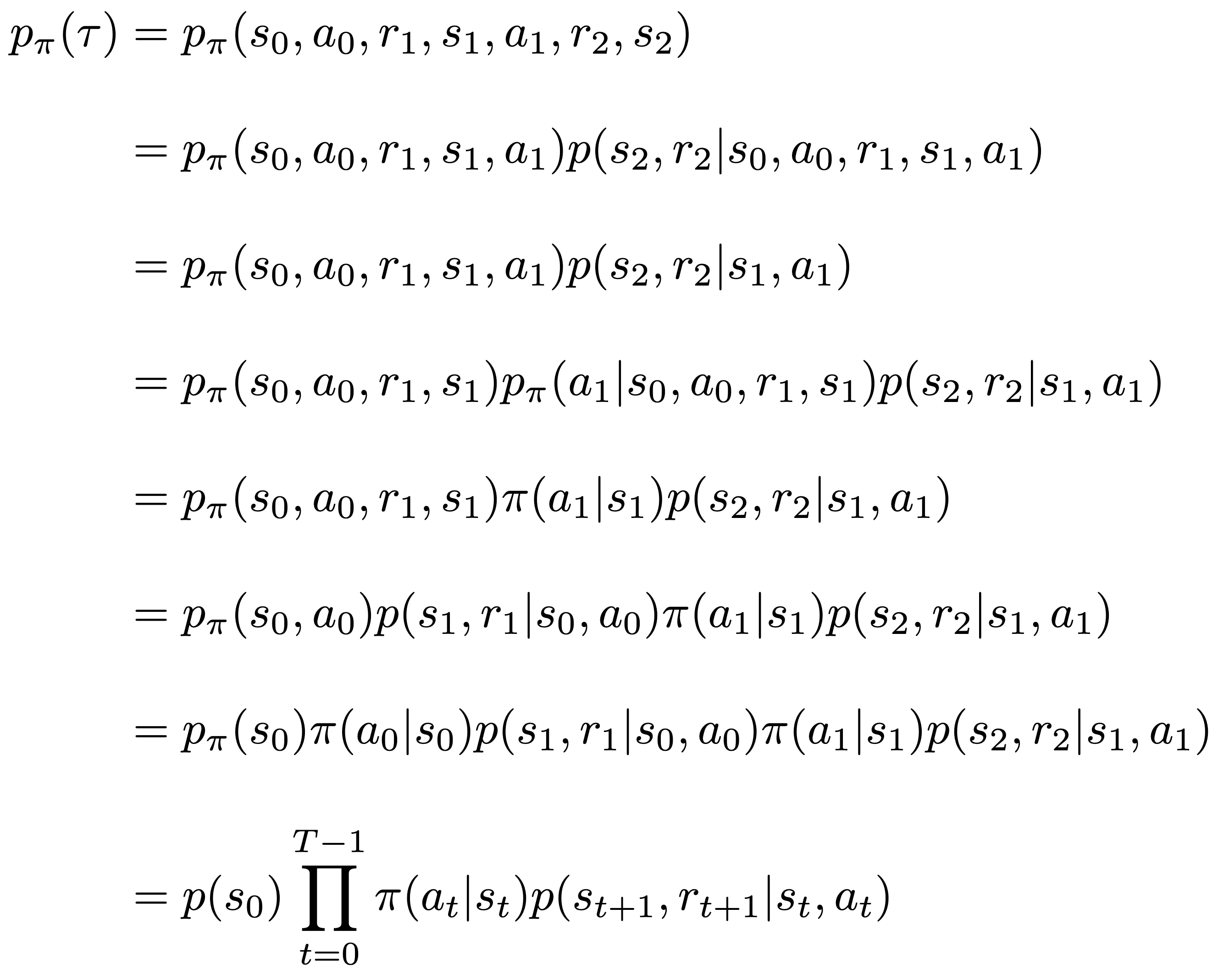
Importance Sampling for Off-Policy Monte-Carlo

➢Goal: estimate

➢Data: trajectory generated with

➢First-step: Compute the probability of a trajectory generated following policy

Definition of conditional probability on
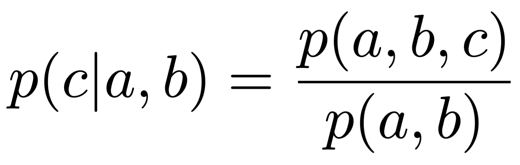
\begin{align*}
p(c|a,b) = \frac{p(a,b,c)}{p(a,b)}
\end{align*}

Markov Property

Def. of conditional probability on

\begin{align*}
p_\pi(\tau) &= p_\pi(s_0, a_0, r_1, s_1, a_1, r_2, s_2) \\[1em] &= p_\pi(s_0, a_0, r_1, s_1, a_1) p(s_2, r_2 | s_0, a_0, r_1, s_1, a_1) \\[1em] &= p_\pi(s_0, a_0, r_1, s_1, a_1) p(s_2, r_2 | s_1, a_1) \\[1em] &= p_\pi(s_0, a_0, r_1, s_1) p_\pi(a_1 | s_0, a_0, r_1, s_1) p(s_2, r_2 | s_1, a_1) \\[1em] &= p_\pi(s_0, a_0, r_1, s_1) \pi(a_1 | s_1) p(s_2, r_2 | s_1, a_1) \\[1em] &= p_\pi(s_0, a_0) p(s_1, r_1 | s_0, a_0) \pi(a_1 | s_1) p(s_2, r_2 | s_1, a_1) \\[1em] &= p_\pi(s_0) \pi(a_0 | s_0) p(s_1, r_1 | s_0, a_0) \pi(a_1 | s_1) p(s_2, r_2 | s_1, a_1) \\[1em] &= p(s_0) \prod_{t=0}^{T-1} \pi(a_t | s_t) p(s_{t+1}, r_{t+1} | s_t, a_t)
\end{align*}
\begin{align*}
p_\pi(\tau) &= p_\pi(s_0, a_0, r_1, s_1, a_1, r_2, s_2) \\[1em] &= p_\pi(s_0, a_0, r_1, s_1, a_1) p(s_2, r_2 | s_0, a_0, r_1, s_1, a_1) \\[1em] &= p_\pi(s_0, a_0, r_1, s_1, a_1) p(s_2, r_2 | s_1, a_1) \\[1em] &= p_\pi(s_0, a_0, r_1, s_1) p_\pi(a_1 | s_0, a_0, r_1, s_1) p(s_2, r_2 | s_1, a_1) \\[1em] &= p_\pi(s_0, a_0, r_1, s_1) \pi(a_1 | s_1) p(s_2, r_2 | s_1, a_1) \\[1em] &= p_\pi(s_0, a_0) p(s_1, r_1 | s_0, a_0) \pi(a_1 | s_1) p(s_2, r_2 | s_1, a_1) \\[1em] &= p_\pi(s_0) \pi(a_0 | s_0) p(s_1, r_1 | s_0, a_0) \pi(a_1 | s_1) p(s_2, r_2 | s_1, a_1) \\[1em] &= p(s_0) \prod_{t=0}^{T-1} \pi(a_t | s_t) p(s_{t+1}, r_{t+1} | s_t, a_t)
\end{align*}
\begin{align*}
p_\pi(\tau) &= p_\pi(s_0, a_0, r_1, s_1, a_1, r_2, s_2) \\[1em] &= p_\pi(s_0, a_0, r_1, s_1, a_1) p(s_2, r_2 | s_0, a_0, r_1, s_1, a_1) \\[1em] &= p_\pi(s_0, a_0, r_1, s_1, a_1) p(s_2, r_2 | s_1, a_1) \\[1em] &= p_\pi(s_0, a_0, r_1, s_1) p_\pi(a_1 | s_0, a_0, r_1, s_1) p(s_2, r_2 | s_1, a_1) \\[1em] &= p_\pi(s_0, a_0, r_1, s_1) \pi(a_1 | s_1) p(s_2, r_2 | s_1, a_1) \\[1em] &= p_\pi(s_0, a_0) p(s_1, r_1 | s_0, a_0) \pi(a_1 | s_1) p(s_2, r_2 | s_1, a_1) \\[1em] &= p_\pi(s_0) \pi(a_0 | s_0) p(s_1, r_1 | s_0, a_0) \pi(a_1 | s_1) p(s_2, r_2 | s_1, a_1) \\[1em] &= p(s_0) \prod_{t=0}^{T-1} \pi(a_t | s_t) p(s_{t+1}, r_{t+1} | s_t, a_t)
\end{align*}
\begin{align*}
p_\pi(\tau) &= p_\pi(s_0, a_0, r_1, s_1, a_1, r_2, s_2) \\[1em] &= p_\pi(s_0, a_0, r_1, s_1, a_1) p(s_2, r_2 | s_0, a_0, r_1, s_1, a_1) \\[1em] &= p_\pi(s_0, a_0, r_1, s_1, a_1) p(s_2, r_2 | s_1, a_1) \\[1em] &= p_\pi(s_0, a_0, r_1, s_1) p_\pi(a_1 | s_0, a_0, r_1, s_1) p(s_2, r_2 | s_1, a_1) \\[1em] &= p_\pi(s_0, a_0, r_1, s_1) \pi(a_1 | s_1) p(s_2, r_2 | s_1, a_1) \\[1em] &= p_\pi(s_0, a_0) p(s_1, r_1 | s_0, a_0) \pi(a_1 | s_1) p(s_2, r_2 | s_1, a_1) \\[1em] &= p_\pi(s_0) \pi(a_0 | s_0) p(s_1, r_1 | s_0, a_0) \pi(a_1 | s_1) p(s_2, r_2 | s_1, a_1) \\[1em] &= p(s_0) \prod_{t=0}^{T-1} \pi(a_t | s_t) p(s_{t+1}, r_{t+1} | s_t, a_t)
\end{align*}
\begin{align*}
p_\pi(\tau) &= p_\pi(s_0, a_0, r_1, s_1, a_1, r_2, s_2) \\[1em] &= p_\pi(s_0, a_0, r_1, s_1, a_1) p(s_2, r_2 | s_0, a_0, r_1, s_1, a_1) \\[1em] &= p_\pi(s_0, a_0, r_1, s_1, a_1) p(s_2, r_2 | s_1, a_1) \\[1em] &= p_\pi(s_0, a_0, r_1, s_1) p_\pi(a_1 | s_0, a_0, r_1, s_1) p(s_2, r_2 | s_1, a_1) \\[1em] &= p_\pi(s_0, a_0, r_1, s_1) \pi(a_1 | s_1) p(s_2, r_2 | s_1, a_1) \\[1em] &= p_\pi(s_0, a_0) p(s_1, r_1 | s_0, a_0) \pi(a_1 | s_1) p(s_2, r_2 | s_1, a_1) \\[1em] &= p_\pi(s_0) \pi(a_0 | s_0) p(s_1, r_1 | s_0, a_0) \pi(a_1 | s_1) p(s_2, r_2 | s_1, a_1) \\[1em] &= p(s_0) \prod_{t=0}^{T-1} \pi(a_t | s_t) p(s_{t+1}, r_{t+1} | s_t, a_t)
\end{align*}
\begin{align*}
p_\pi(\tau) &= p_\pi(s_0, a_0, r_1, s_1, a_1, r_2, s_2) \\[1em] &= p_\pi(s_0, a_0, r_1, s_1, a_1) p(s_2, r_2 | s_0, a_0, r_1, s_1, a_1) \\[1em] &= p_\pi(s_0, a_0, r_1, s_1, a_1) p(s_2, r_2 | s_1, a_1) \\[1em] &= p_\pi(s_0, a_0, r_1, s_1) p_\pi(a_1 | s_0, a_0, r_1, s_1) p(s_2, r_2 | s_1, a_1) \\[1em] &= p_\pi(s_0, a_0, r_1, s_1) \pi(a_1 | s_1) p(s_2, r_2 | s_1, a_1) \\[1em] &= p_\pi(s_0, a_0) p(s_1, r_1 | s_0, a_0) \pi(a_1 | s_1) p(s_2, r_2 | s_1, a_1) \\[1em] &= p_\pi(s_0) \pi(a_0 | s_0) p(s_1, r_1 | s_0, a_0) \pi(a_1 | s_1) p(s_2, r_2 | s_1, a_1) \\[1em] &= p(s_0) \prod_{t=0}^{T-1} \pi(a_t | s_t) p(s_{t+1}, r_{t+1} | s_t, a_t)
\end{align*}
\begin{align*}
p_\pi(\tau) &= p_\pi(s_0, a_0, r_1, s_1, a_1, r_2, s_2) \\[1em] &= p_\pi(s_0, a_0, r_1, s_1, a_1) p(s_2, r_2 | s_0, a_0, r_1, s_1, a_1) \\[1em] &= p_\pi(s_0, a_0, r_1, s_1, a_1) p(s_2, r_2 | s_1, a_1) \\[1em] &= p_\pi(s_0, a_0, r_1, s_1) p_\pi(a_1 | s_0, a_0, r_1, s_1) p(s_2, r_2 | s_1, a_1) \\[1em] &= p_\pi(s_0, a_0, r_1, s_1) \pi(a_1 | s_1) p(s_2, r_2 | s_1, a_1) \\[1em] &= p_\pi(s_0, a_0) p(s_1, r_1 | s_0, a_0) \pi(a_1 | s_1) p(s_2, r_2 | s_1, a_1) \\[1em] &= p_\pi(s_0) \pi(a_0 | s_0) p(s_1, r_1 | s_0, a_0) \pi(a_1 | s_1) p(s_2, r_2 | s_1, a_1) \\[1em] &= p(s_0) \prod_{t=0}^{T-1} \pi(a_t | s_t) p(s_{t+1}, r_{t+1} | s_t, a_t)
\end{align*}
\begin{align*}
p_\pi(\tau) &= p_\pi(s_0, a_0, r_1, s_1, a_1, r_2, s_2) \\[1em] &= p_\pi(s_0, a_0, r_1, s_1, a_1) p(s_2, r_2 | s_0, a_0, r_1, s_1, a_1) \\[1em] &= p_\pi(s_0, a_0, r_1, s_1, a_1) p(s_2, r_2 | s_1, a_1) \\[1em] &= p_\pi(s_0, a_0, r_1, s_1) p_\pi(a_1 | s_0, a_0, r_1, s_1) p(s_2, r_2 | s_1, a_1) \\[1em] &= p_\pi(s_0, a_0, r_1, s_1) \pi(a_1 | s_1) p(s_2, r_2 | s_1, a_1) \\[1em] &= p_\pi(s_0, a_0) p(s_1, r_1 | s_0, a_0) \pi(a_1 | s_1) p(s_2, r_2 | s_1, a_1) \\[1em] &= p_\pi(s_0) \pi(a_0 | s_0) p(s_1, r_1 | s_0, a_0) \pi(a_1 | s_1) p(s_2, r_2 | s_1, a_1) \\[1em] &= p(s_0) \prod_{t=0}^{T-1} \pi(a_t | s_t) p(s_{t+1}, r_{t+1} | s_t, a_t)
\end{align*}

Importance Sampling for Off-Policy Monte-Carlo

➢Goal: estimate

➢Data: trajectory generated with

➢First-step: Compute the probability of a trajectory generated following policy
Definition of conditional probability on

\begin{align*}
p(c|a,b) = \frac{p(a,b,c)}{p(a,b)}
\end{align*}

Markov Property

Def. of conditional probability on

Definition of policy (“It is Markov”)

Conditional probability on

Definition of policy on

General formulation for trajectories until Terminal state.

\begin{align*}
p_\pi(\tau) &= p_\pi(s_0, a_0, r_1, s_1, a_1, r_2, s_2) \\[1em] &= p_\pi(s_0, a_0, r_1, s_1, a_1) p(s_2, r_2 | s_0, a_0, r_1, s_1, a_1) \\[1em] &= p_\pi(s_0, a_0, r_1, s_1, a_1) p(s_2, r_2 | s_1, a_1) \\[1em] &= p_\pi(s_0, a_0, r_1, s_1) p_\pi(a_1 | s_0, a_0, r_1, s_1) p(s_2, r_2 | s_1, a_1) \\[1em] &= p_\pi(s_0, a_0, r_1, s_1) \pi(a_1 | s_1) p(s_2, r_2 | s_1, a_1) \\[1em] &= p_\pi(s_0, a_0) p(s_1, r_1 | s_0, a_0) \pi(a_1 | s_1) p(s_2, r_2 | s_1, a_1) \\[1em] &= p_\pi(s_0) \pi(a_0 | s_0) p(s_1, r_1 | s_0, a_0) \pi(a_1 | s_1) p(s_2, r_2 | s_1, a_1) \\[1em] &= p(s_0) \prod_{t=0}^{T-1} \pi(a_t | s_t) p(s_{t+1}, r_{t+1} | s_t, a_t)
\end{align*}

Importance Sampling for Off-Policy Monte-Carlo

➢Goal: estimate

➢Data: trajectory generated with

➢First-step: Compute the probability of a trajectory generated following policy

\begin{align*}
p_\pi(\tau) &= p_\pi(s_0, a_0, r_1, s_1, a_1, r_2, s_2) \\[1em] &= p_\pi(s_0, a_0, r_1, s_1, a_1) p(s_2, r_2 | s_0, a_0, r_1, s_1, a_1) \\[1em] &= p_\pi(s_0, a_0, r_1, s_1, a_1) p(s_2, r_2 | s_1, a_1) \\[1em] &= p_\pi(s_0, a_0, r_1, s_1) p_\pi(a_1 | s_0, a_0, r_1, s_1) p(s_2, r_2 | s_1, a_1) \\[1em] &= p_\pi(s_0, a_0, r_1, s_1) \pi(a_1 | s_1) p(s_2, r_2 | s_1, a_1) \\[1em] &= p_\pi(s_0, a_0) p(s_1, r_1 | s_0, a_0) \pi(a_1 | s_1) p(s_2, r_2 | s_1, a_1) \\[1em] &= p_\pi(s_0) \pi(a_0 | s_0) p(s_1, r_1 | s_0, a_0) \pi(a_1 | s_1) p(s_2, r_2 | s_1, a_1) \\[1em] &= p(s_0) \prod_{t=0}^{T-1} \pi(a_t | s_t) p(s_{t+1}, r_{t+1} | s_t, a_t)
\end{align*}

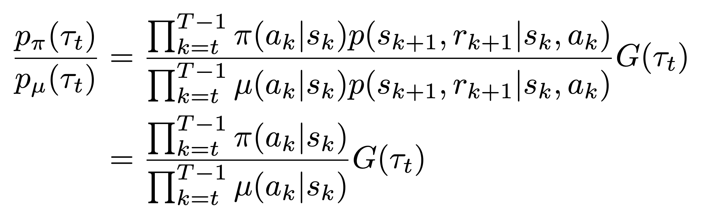
Importance Sampling for Off-Policy Monte-Carlo

➢Goal: estimate

➢Data: trajectory generated with

➢First-step: Compute the probability of a trajectory generated following policy

\begin{align*}
\frac{p_\pi(\tau_t)}{p_\mu(\tau_t)} G(\tau_t) &= \frac{\prod_{k=t}^{T-1} \pi(a_k | s_k) p(s_{k+1}, r_{k+1} | s_k, a_k)}{\prod_{k=t}^{T-1} \mu(a_k | s_k) p(s_{k+1}, r_{k+1} | s_k, a_k)} G(\tau_t) \\ &= \frac{\prod_{k=t}^{T-1} \pi(a_k | s_k)}{\prod_{k=t}^{T-1} \mu(a_k | s_k)} G(\tau_t)
\end{align*}

➢Solution: use return , and correct:

\begin{align*}
\frac{p_\pi(\tau_t)}{p_\mu(\tau_t)} G(\tau_t) &= \frac{\prod_{k=t}^{T-1} \pi(a_k | s_k) p(s_{k+1}, r_{k+1} | s_k, a_k)}{\prod_{k=t}^{T-1} \mu(a_k | s_k) p(s_{k+1}, r_{k+1} | s_k, a_k)} G(\tau_t) \\ &= \frac{\prod_{k=t}^{T-1} \pi(a_k | s_k)}{\prod_{k=t}^{T-1} \mu(a_k | s_k)} G(\tau_t)
\end{align*}
\begin{align*}
p_\pi(\tau) &= p_\pi(s_0, a_0, r_1, s_1, a_1, r_2, s_2) \\[1em] &= p_\pi(s_0, a_0, r_1, s_1, a_1) p(s_2, r_2 | s_0, a_0, r_1, s_1, a_1) \\[1em] &= p_\pi(s_0, a_0, r_1, s_1, a_1) p(s_2, r_2 | s_1, a_1) \\[1em] &= p_\pi(s_0, a_0, r_1, s_1) p_\pi(a_1 | s_0, a_0, r_1, s_1) p(s_2, r_2 | s_1, a_1) \\[1em] &= p_\pi(s_0, a_0, r_1, s_1) \pi(a_1 | s_1) p(s_2, r_2 | s_1, a_1) \\[1em] &= p_\pi(s_0, a_0) p(s_1, r_1 | s_0, a_0) \pi(a_1 | s_1) p(s_2, r_2 | s_1, a_1) \\[1em] &= p_\pi(s_0) \pi(a_0 | s_0) p(s_1, r_1 | s_0, a_0) \pi(a_1 | s_1) p(s_2, r_2 | s_1, a_1) \\[1em] &= p(s_0) \prod_{t=0}^{T-1} \pi(a_t | s_t) p(s_{t+1}, r_{t+1} | s_t, a_t)
\end{align*}
\begin{align*}
p_\pi(\tau) &= p_\pi(s_0, a_0, r_1, s_1, a_1, r_2, s_2) \\[1em] &= p_\pi(s_0, a_0, r_1, s_1, a_1) p(s_2, r_2 | s_0, a_0, r_1, s_1, a_1) \\[1em] &= p_\pi(s_0, a_0, r_1, s_1, a_1) p(s_2, r_2 | s_1, a_1) \\[1em] &= p_\pi(s_0, a_0, r_1, s_1) p_\pi(a_1 | s_0, a_0, r_1, s_1) p(s_2, r_2 | s_1, a_1) \\[1em] &= p_\pi(s_0, a_0, r_1, s_1) \pi(a_1 | s_1) p(s_2, r_2 | s_1, a_1) \\[1em] &= p_\pi(s_0, a_0) p(s_1, r_1 | s_0, a_0) \pi(a_1 | s_1) p(s_2, r_2 | s_1, a_1) \\[1em] &= p_\pi(s_0) \pi(a_0 | s_0) p(s_1, r_1 | s_0, a_0) \pi(a_1 | s_1) p(s_2, r_2 | s_1, a_1) \\[1em] &= p(s_0) \prod_{t=0}^{T-1} \pi(a_t | s_t) p(s_{t+1}, r_{t+1} | s_t, a_t)
\end{align*}

Importance Sampling for Off-Policy TD Updates

➢Use TD targets generated from to evaluate

​

➢Weigh TD target by importance sampling

​

➢Only need a single importance sampling correction

➢Much lower variance than Monte-Carlo importance sampling

​

➢Policies only need to be similar over a single step

\begin{align*}
     v(S_t) \leftarrow v(S_t) + \alpha \Big( {\color{blue}\frac{\pi(A_t|S_t)}{\mu(A_t|S_t)}(R_{t+1} + \gamma v(S_{t+1}))} - v(S_t) \Big) 
\end{align*}

Importance Sampling for Off-Policy TD Updates (Proof)

\begin{align*}
    \mathbb{E}_{\mu} \Big[\frac{\pi(A_t|S_t)}{\mu(A_t|S_t)}(R_{t+1} + \gamma v(S_{t+1})) - v(S_t) \Big| S_t = s \Big]   
\end{align*}
\begin{align*}
    = \sum_a \mu(a|s) \Big(\frac{\pi(a|s)}{\mu(a|s)} \mathbb{E}[R_{t+1} + \gamma v(S_{t+1})|S_t = s, A_t = a] - v(s) \Big) 
\end{align*}
\begin{align*}
    = \sum_a \pi(a|s) \mathbb{E}[R_{t+1} + \gamma v(S_{t+1})|S_t = s, A_t = a] - \sum_a \mu(a|s) v(s) 
\end{align*}
\begin{align*}
    = \sum_a \pi(a|s) \mathbb{E}[R_{t+1} + \gamma v(S_{t+1})|S_t = s, A_t = a] - \sum_a \pi(a|s) v(s) 
\end{align*}
\begin{align*}
    = \sum_a \pi(a|s) \Big(\mathbb{E}[R_{t+1} + \gamma v(S_{t+1})|S_t = s, A_t = a] -  v(s) \Big) 
\end{align*}
\begin{align*}
   = \mathbb{E}_{\pi}\Big[R_{t+1} + \gamma v(S_{t+1}) - v(s)|S_t = s\Big]  
\end{align*}

Take home message

•Q-learning uses a greedy target policy

•SARSA uses a stochastic sample from the behaviour as target policy

•Expected SARSA uses any target policy

•Double learning uses a separate value function to evaluate the policy

•Double learning is not necessary if there is no correlation between target policy
and value function.

•When using a greedy policy (Q-learning), there are strong correlations. Then
double learning (Double Q-learning) can be useful.

•DQN is q-learning with function approximation on the state space plus replay
buffer and target network to help stabilize training.

​

Take home message