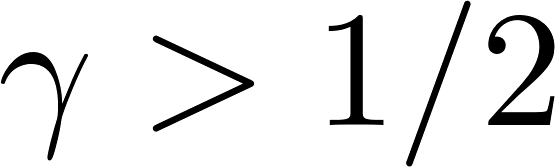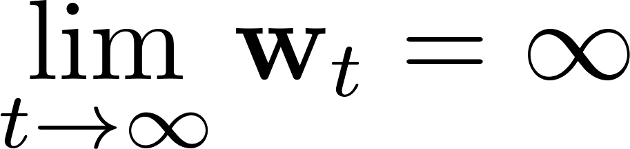


Reinforcement Learning · Lecture 6
Function Approximation
Rafael Fernandes Cunha

Today’s topics
1.Recap Model-Free Control
2.Value Function approximation (VFA)
3.Classes of VFA
1.Tabular
2.State Aggregation
3.Linear
4.Non-linear
4.Stochastic Gradient Descent (SGD) with VFA
5.Linear VFA
6.Prediction and Control with VFA
2
1.Describe the different types of VFA
2.Apply the SGD algorithm to a linear VFA
3.Explain what feature vectors are
4.Explain the VFA update expression for MC, TD
and SARSA methods
5.Explain why TD is not a true SGD algorithm
Learning outcomes
Behaviour vs Target policy
Behavior policy: Generate the action the agent will actually perform in the environment.
Target policy: The policy we want to learn.
Behaviour vs Target policy
The simulation is currently at state
Which policy
➢… chooses the action that the agent will actually perform in the environment?
➢… leads the environment to produce and ?
➢… generates the action used solely for estimation?
➢… determines how to evaluate the next state , for the learning update ?
➢… defines the action-value function is used to compute ?
➢… is the policy we are trying to learn and improve?
➢… needs to ensure sufficient exploration?
➢… defines the Bellman expectation equations?
Approach to ensure all actions are selected infinitely often
On-policy: Learn about target policy from experience sampled from behaviour policy
Off-policy: Learn about target policy from experience sampled from behaviour policy
target policy = behaviour policy
target policy behaviour policy
Action-value update equations
Correct or Wrong?
✅
❌
✅
❌
SARSA vs Q-learning
greedy
-greedy
SARSA (Behavior policy = Target policy)
Q-learning
Policy must be GLIE to assure convergence.
Behaviour policy should provide infinite exploration.

Q-learning overestimation and Double q-learning
Selecting the action
Evaluating the action
Q-learning overestimates because:
1) It uses the same action-value function to select and to evaluate the action!
2) It has the maximization term.

![\begin{align*}
\textcolor{blue}{q_2}(S_t, A_t) \leftarrow \textcolor{blue}{q_2}(S_t, A_t) + \alpha \big[R_{t+1} + \gamma \textcolor{red}{q_1}\Big(S_{t+1}, \argmax_a \textcolor{blue}{q_2}(S_{t+1}, a)\Big) - \textcolor{blue}{q_2}(S_t, A_t)\Big]
\end{align*}](media/a89a6088ec.png)
![\begin{align*}
\textcolor{red}{q_1}(S_t, A_t) \leftarrow \textcolor{red}{q_1}(S_t, A_t) + \alpha \big[R_{t+1} + \gamma \textcolor{blue}{q_2}\Big(S_{t+1}, \argmax_a \textcolor{red}{q_1}(S_{t+1}, a)\Big) - \textcolor{red}{q_1}(S_t, A_t)\Big]
\end{align*}](media/b1db6d6709.png)
DQN
Q-learning with tricks to help convergence
➢Replay Buffer: Sampling from this buffer helps get less correlated data.
➢Target Network: Avoid chasing a moving target
Off-Policy Learning: Importance Sampling Corrections
Off-policy: Learn about target policy from experience sampled from behaviour policy
Evaluate target policy
to compute or
Use behaviour policy
to generate actions
➢Note that you are sampling from one probability distribution to learn about a different one.

![\begin{align*}
\mathbb{E}[R_{t+1}|S_t = s, A_t \sim \pi]
\end{align*}](media/c32a33fb6b.png)
![\begin{align*}
= \mathbb{E} \Big[\frac{\pi(A_t|S_t)}{\mu(A_t|S_t)}R_{t+1} | S_t = s, A_t \sim \mu \Big]
\end{align*}](media/8fad1d714d.png)
Incremental Update rule
NewEstimate
OldEstimate
StepSize
InformativeValue
Estimate
Target
OldEstimate
-
Control:
Each algorithm changes only the Target value!
Algorithms: Model-Free Control
Monte Carlo
SARSA
Q-learning
Expected SARSA
Double Q-learning
Greedy policy
Algorithms: Model-Free Control
Monte Carlo
SARSA
Q-learning
Expected SARSA
Double Q-learning
Greedy policy
Function Approximation
Today’s lecture!
Function Approximation
➢The policy, value function, and model, are all functions.
➢We want to learn these from experience.
➢If there are too many states, we need to approximate.
We consider learning predictions (value functions; including value-based control)
Why function approximation?
Large-Scale Reinforcement Learning
Reinforcement learning can be used to solve large problems, e.g.
➢Backgammon: states
➢Go: states
➢Helicopter: continuous state space
➢Robots: real world
How can we apply our methods for prediction and control?
Value function approximation
So far we mostly considered lookup tables
➢Every state s has an entry v(s)
➢Or every state-action pair has an entry
Problem with large MDPs:
➢There are too many states and/or actions to store in memory
➢It is too slow to learn the value of each state individually
➢Individual environment states are often not fully observable
Value function approximation
Solution for large MDPs
Estimate value function with function approximation.


Update parameter w
How?
Using MC or TD learning.
Generalize to unseen states
Classes of Function Approximation
➢Tabular: a table with an entry for each MDP state
➢State aggregation: Partition environment states (or observations) into a discrete set
➢Linear function approximation
➢Consider fixed agent state update (e.g., )
➢Fixed feature map
➢Values are linear function of features:
➢Note: state aggregation and tabular are special cases of linear FA
➢Differentiable function approximation
➢ is a differentiable function of w, could be non-linear
➢E.g., a convolutional neural network that takes pixels as input
➢Another interpretation: features are not fixed, but learned
Classes of Function Approximation
In principle, any function approximator can be used, but RL has specific properties:
➢Experience is not i.i.d. — successive time-steps are correlated
➢Agent’s policy affects the data it receives
➢Regression targets can be non-stationary
➢...because of changing policies (which can change the target and the data!)
➢...because of bootstrapping
➢...because of non-stationary dynamics (e.g., other learning agents)
➢...because the world is large (never quite in the same state)
Classes of Function Approximation
Which function approximation should you choose?
Tabular: good theory but does not scale/generalize
Linear: reasonably good theory, but requires good features
Non-linear: less well-understood, but scales well
➢Flexible, and less reliant on picking good features first (e.g., by hand)
➢(Deep) neural nets often perform quite well, and remain a popular choice
Approximate Values By Stochastic Gradient Descent
Goal: Learn the state-value function

![\begin{align*}
J(\mathbf{w}) = \mathbb{E}_{S \sim d}[(v_{\pi}(S) - v_{\mathbf{w}}(S))^2]
\end{align*}](media/a521b77bc8.png)
True value
![\begin{align*}
J(\mathbf{w}) = \mathbb{E}_{S \sim d}[(v_{\pi}(S) - v_{\mathbf{w}}(S))^2]
\end{align*}](media/a521b77bc8.png)
Estimated value
parameterized by w
![\begin{align*}
J(\mathbf{w}) = \mathbb{E}_{S \sim d}[(v_{\pi}(S) - v_{\mathbf{w}}(S))^2]
\end{align*}](media/a521b77bc8.png)
Approximate Values By Stochastic Gradient Descent
![\begin{align*}
J(\mathbf{w}) = \mathbb{E}_{S \sim d}[(v_{\pi}(S) - v_{\mathbf{w}}(S))^2]
\end{align*}](media/a521b77bc8.png)
Goal: Learn the state-value function
![\begin{align*}
J(\mathbf{w}) = \mathbb{E}_{S \sim d}[(v_{\pi}(S) - v_{\mathbf{w}}(S))^2]
\end{align*}](media/a521b77bc8.png)
True value
Estimated value
parameterized by w
![\begin{align*}
J(\mathbf{w}) = \mathbb{E}_{S \sim d}[(v_{\pi}(S) - v_{\mathbf{w}}(S))^2]
\end{align*}](media/a521b77bc8.png)
![\begin{align*}
J(\mathbf{w}) = \mathbb{E}_{S \sim d}[(v_{\pi}(S) - v_{\mathbf{w}}(S))^2]
\end{align*}](media/a521b77bc8.png)
Loss function
Approximate Values By Stochastic Gradient Descent
![\begin{align*}
J(\mathbf{w}) = \mathbb{E}_{S \sim d}[(v_{\pi}(S) - v_{\mathbf{w}}(S))^2]
\end{align*}](media/a521b77bc8.png)
Goal: Learn the state-value function
Find w that minimize this difference!
Goal:
Approximate Values By Stochastic Gradient Descent
![\begin{align*}
J(\mathbf{w}) = \mathbb{E}_{S \sim d}[(v_{\pi}(S) - v_{\mathbf{w}}(S))^2]
\end{align*}](media/a521b77bc8.png)
Goal: Learn the state-value function
Let it be a differentiable
function of parameter vector w
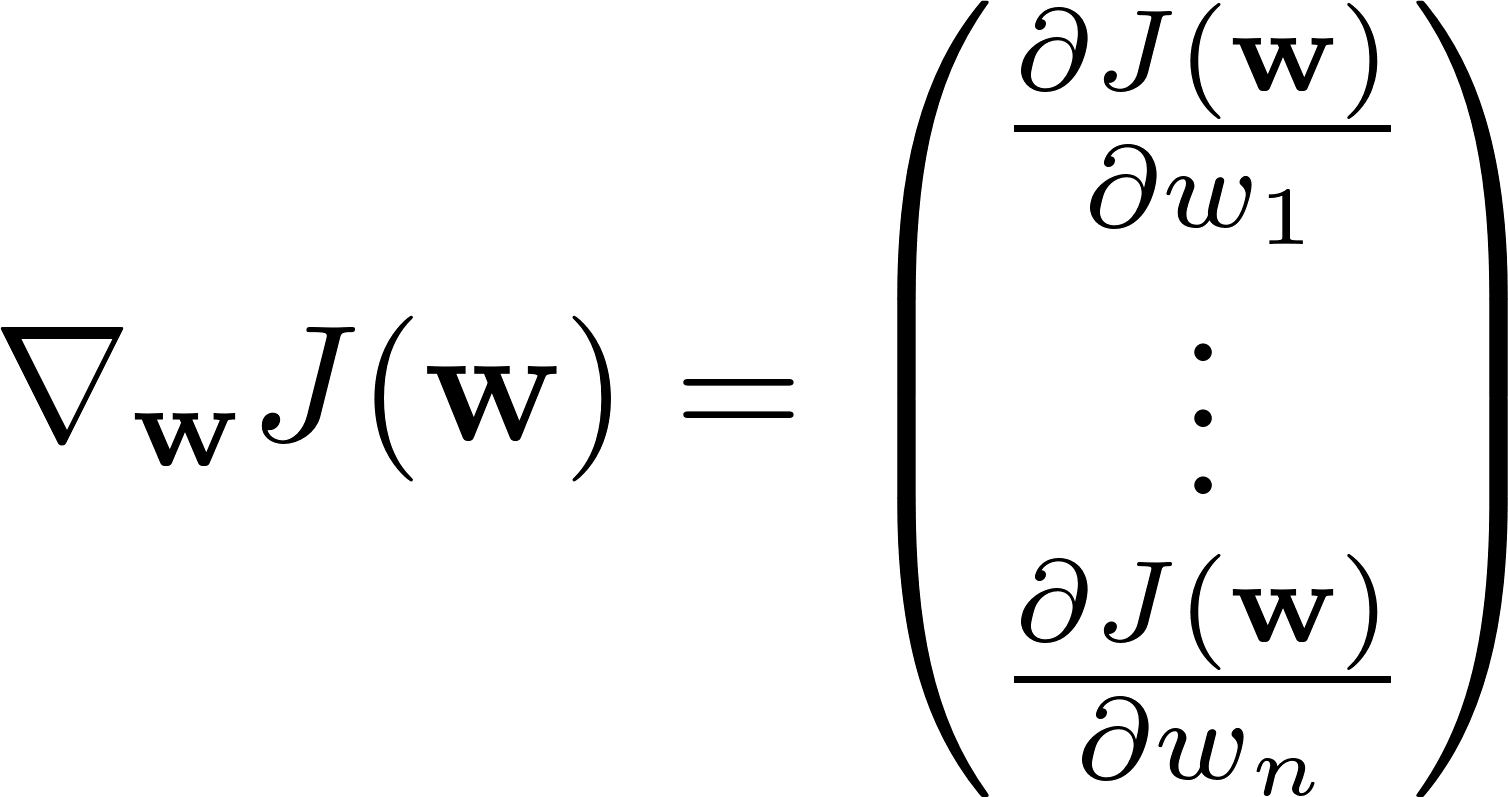
Gradient
Goal: to minimize
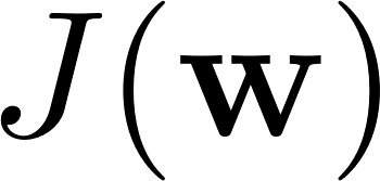
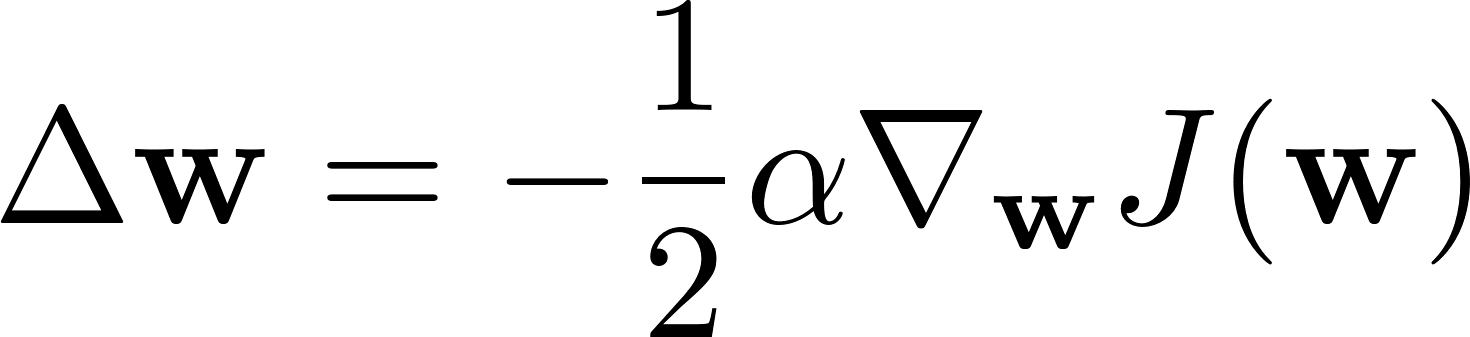
Method: move w in the direction of negative gradient
step-size parameter
Update rule:

Approximate Values By Stochastic Gradient Descent
![\begin{align*}
J(\mathbf{w}) = \mathbb{E}_{S \sim d}[(v_{\pi}(S) - v_{\mathbf{w}}(S))^2]
\end{align*}](media/a521b77bc8.png)
Goal: Learn the state-value function


Approximate Values By Stochastic Gradient Descent
![\begin{align*}
J(\mathbf{w}) = \mathbb{E}_{S \sim d}[(v_{\pi}(S) - v_{\mathbf{w}}(S))^2]
\end{align*}](media/a521b77bc8.png)
Goal: Learn the state-value function


How to solve it without a model?
This is an expectation equation.
We need to sample it!
Stochastic Gradient Descent


![\begin{align*}
=- \frac{1}{2} \alpha \Big(2 \mathbb{E}_{S \sim d}[v_{\pi}(S) - v_{\mathbf{w}}(S)] \nabla_{\mathbf{w}} \big(v_{\pi}(S) -v_{\mathbf{w}}(S) \big) \Big)\\
\end{align*}](media/12a5e69c1b.png)
![\begin{align*}
=- \alpha \mathbb{E}_{S \sim d}[v_{\pi}(S) - v_{\mathbf{w}}(S)] \Big(\nabla_{\mathbf{w}} v_{\pi}(S) -\nabla_{\mathbf{w}}v_{\mathbf{w}}(S) \Big)
\end{align*}](media/1065eb4bae.png)
![\begin{align*}
= \alpha \mathbb{E}_{S \sim d}[v_{\pi}(S) - v_{\mathbf{w}}(S)] \nabla_{\mathbf{w}}v_{\mathbf{w}}(S)
\end{align*}](media/cfb9fea374.png)
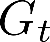
Monte Carlo:
TD(0):
TD():


Approximate Values By Stochastic Gradient Descent
![\begin{align*}
J(\mathbf{w}) = \mathbb{E}_{S \sim d}[(v_{\pi}(S) - v_{\mathbf{w}}(S))^2]
\end{align*}](media/a521b77bc8.png)
Goal: Learn the state-value function


Stochastic Gradient Descent
How do we approximate the true
(target) value when sampling?
Monte Carlo:
TD(0):
TD():


Approximate Values By Stochastic Gradient Descent
![\begin{align*}
J(\mathbf{w}) = \mathbb{E}_{S \sim d}[(v_{\pi}(S) - v_{\mathbf{w}}(S))^2]
\end{align*}](media/a521b77bc8.png)
Goal: Learn the state-value function


Stochastic Gradient Descent
Do you see any problem here?

Monte Carlo:
TD(0):
TD():


Approximate Values By Stochastic Gradient Descent
![\begin{align*}
J(\mathbf{w}) = \mathbb{E}_{S \sim d}[(v_{\pi}(S) - v_{\mathbf{w}}(S))^2]
\end{align*}](media/a521b77bc8.png)
Goal: Learn the state-value function


Stochastic Gradient Descent
Do you see any problem here?

We considered that did not depend
on w when taking the gradient!
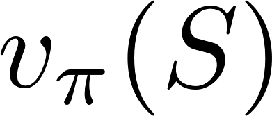

TD(0):
TD():


Approximate Values By Stochastic Gradient Descent
![\begin{align*}
J(\mathbf{w}) = \mathbb{E}_{S \sim d}[(v_{\pi}(S) - v_{\mathbf{w}}(S))^2]
\end{align*}](media/a521b77bc8.png)
Goal: Learn the state-value function


Stochastic Gradient Descent
Do you see any problem here?

We considered that did not depend
on w when taking the gradient!

Bootstrapping methods are biased! They do not produce a true gradient-descent method!
They include only a part of the gradient. We call them semi-gradient methods.
Approximate Values By Stochastic Gradient Descent
![\begin{align*}
J(\mathbf{w}) = \mathbb{E}_{S \sim d}[(v_{\pi}(S) - v_{\mathbf{w}}(S))^2]
\end{align*}](media/a521b77bc8.png)
Goal: Learn the state-value function


Stochastic Gradient Descent
How to compute this gradient?
Linear
Non-linear
We need to define how we are approximating our function!
(Deep) neural nets
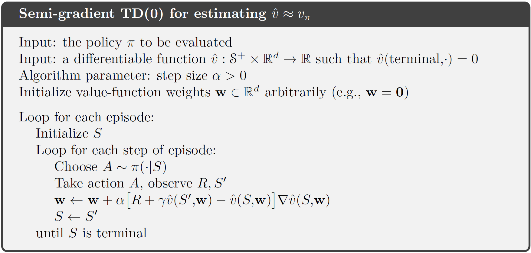
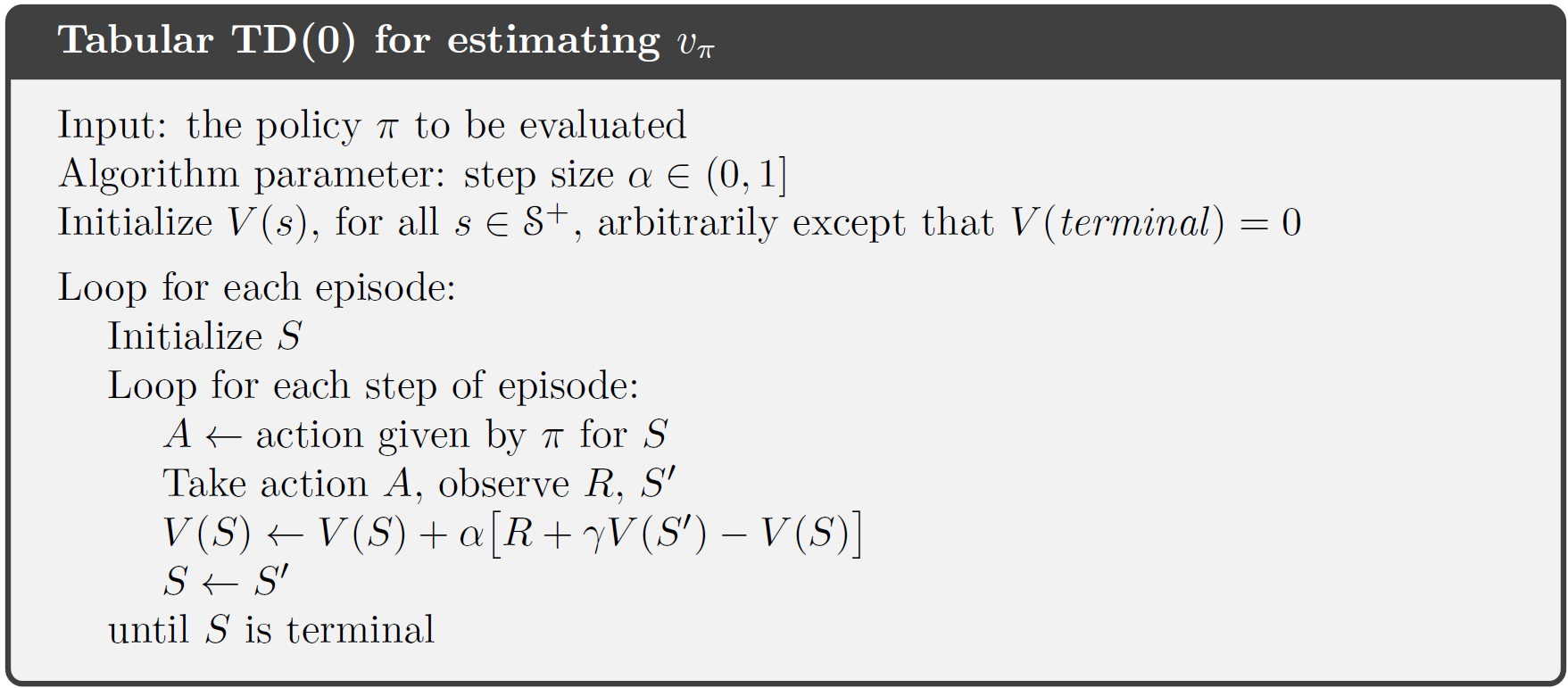

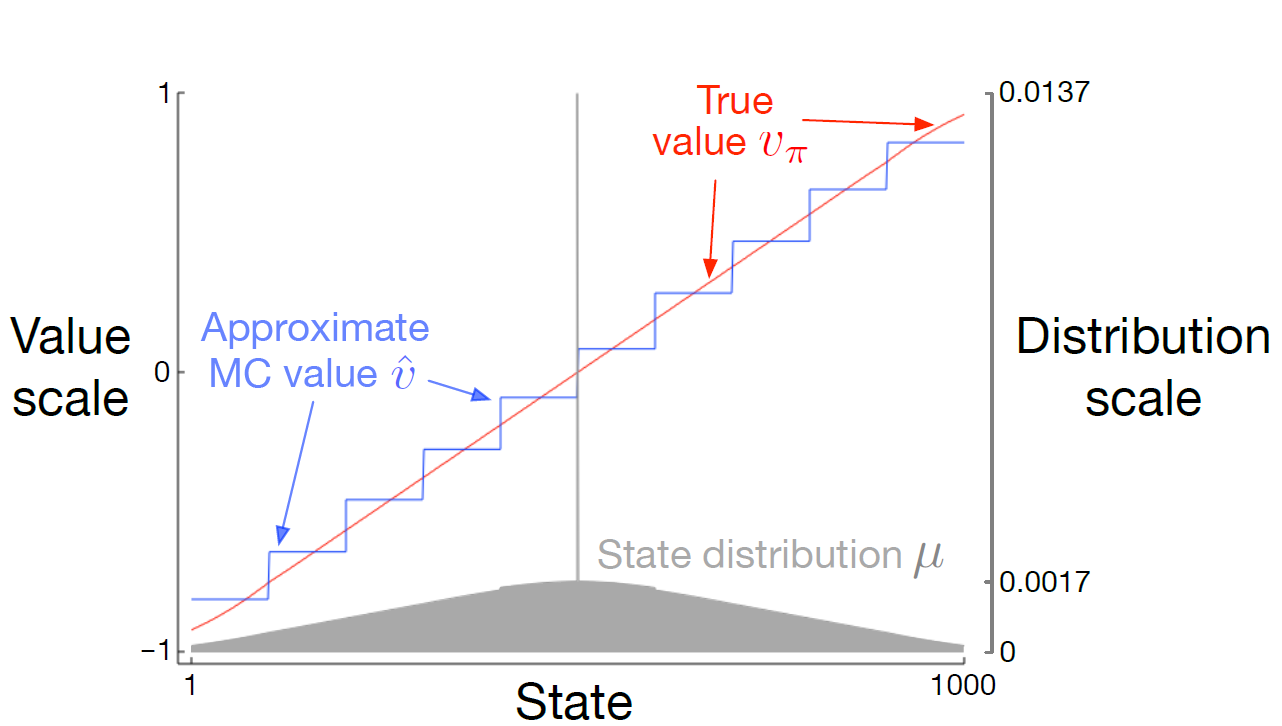
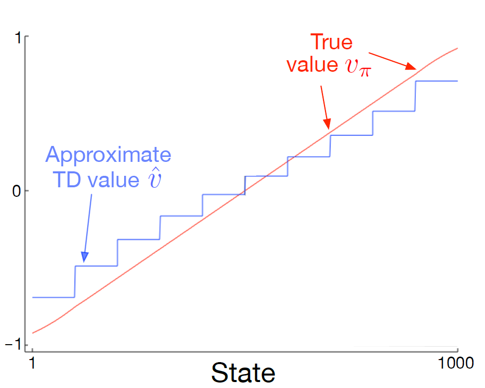
Example: 1000-state random walk task



Asymptotic values of semi-gradient TD are worse than the asymptotic Monte Carlo values.
Action-Value Function Approximation
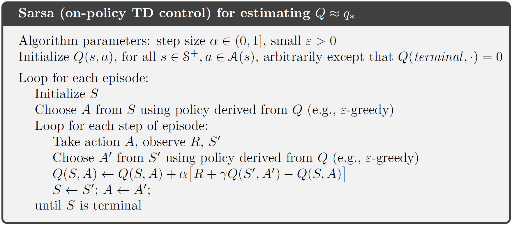
SARSA is TD applied to state-action pairs

![\begin{align*}
\mathbf{w}_{t+1} \doteq \mathbf{w}_t + \alpha \Big[ q_{\pi}(s,a) - q_{\mathbf{w}_t}(S_t, A_t)\Big] \nabla q_{\mathbf{w}_t}(S_t, A_t)
\end{align*}](media/b56cceed8d.png)
![\begin{align*}
\mathbf{w}_{t+1} \doteq \mathbf{w}_t + \alpha \Big[{\color{blue}R_{t+1} + \gamma q_{\mathbf{w}_t}(S_{t+1}, A_{t+1})}- q_{\mathbf{w}}(S_t, A_t)\Big] \nabla q_{\mathbf{w}_t}(S_t, A_t)
\end{align*}](media/a47df3cac6.png)
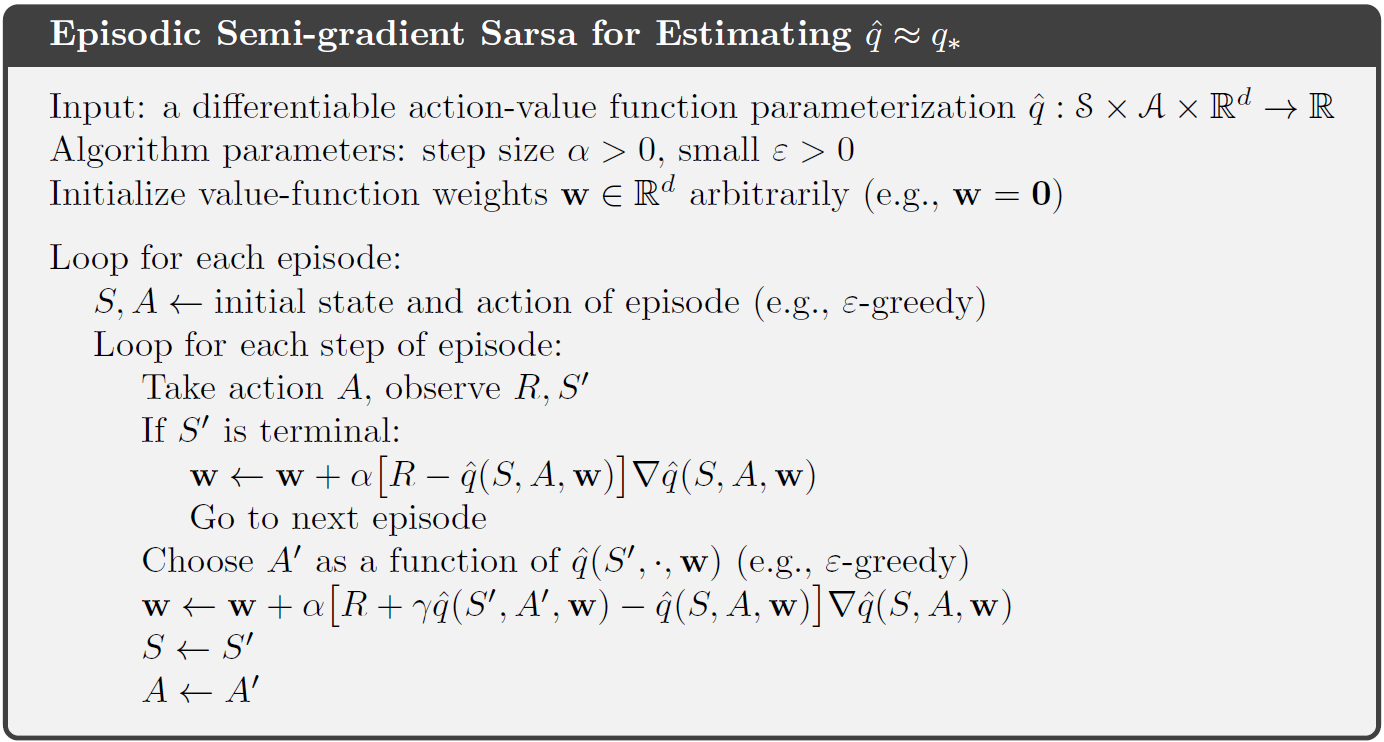
Episodic semi-gradient one-step SARSA


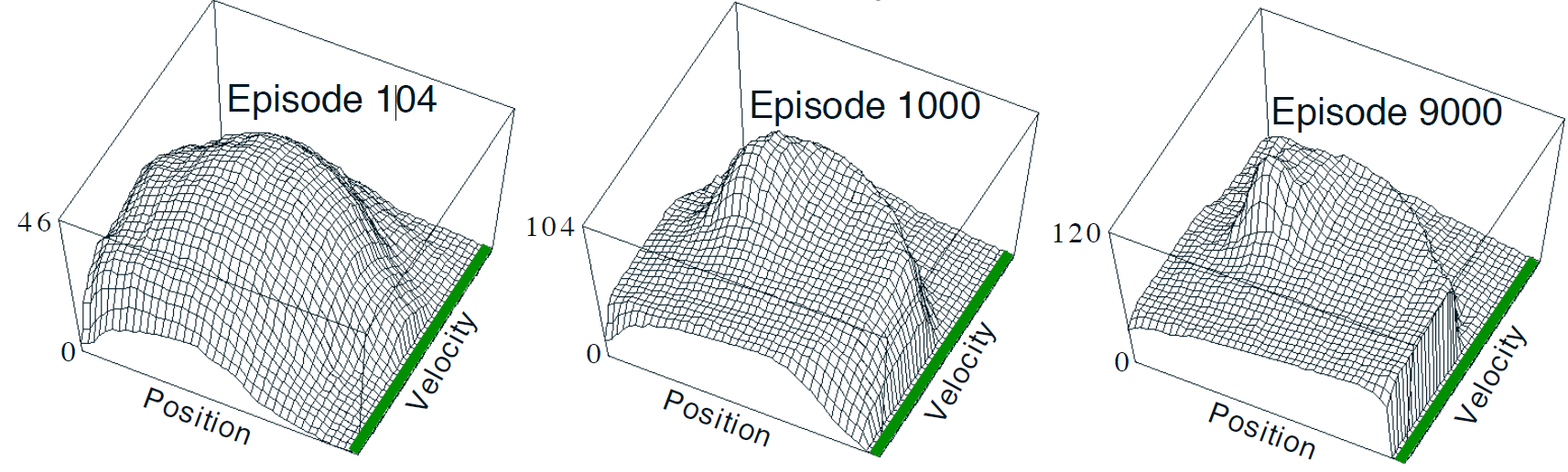
Example: Mountain Car Task (semi-gradient SARSA())
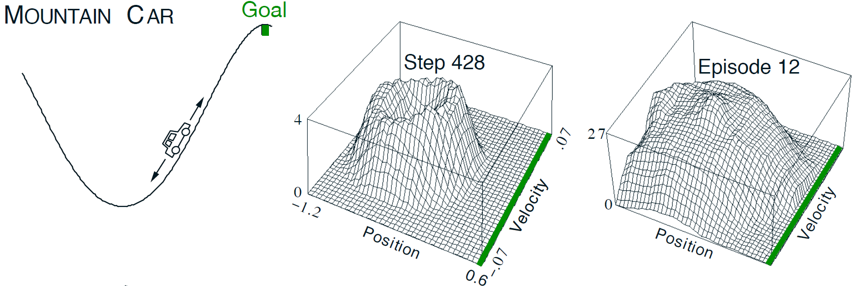


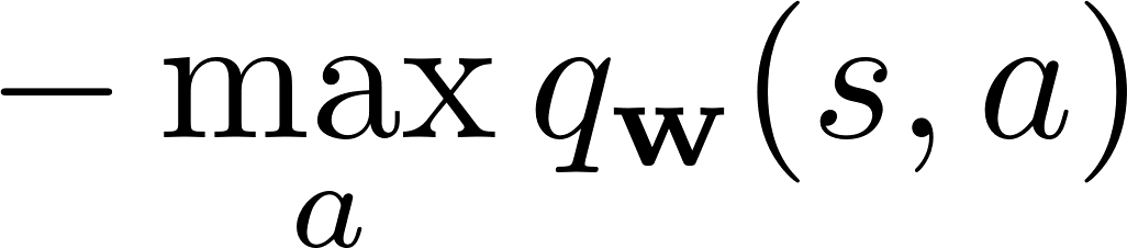
Cost-to-go
Linear Function Approximation


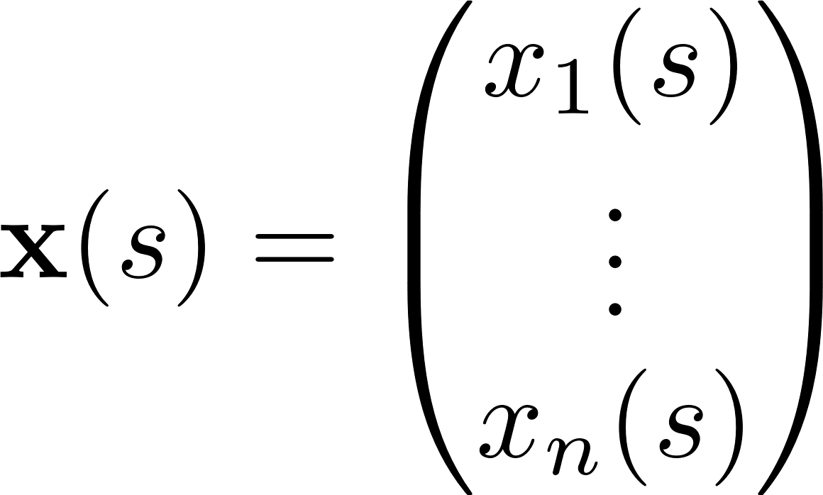
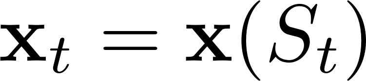
Represent state by a feature vector
is a fixed mapping from state to features
Short-hand:
Examples:
➢Distance of robot from landmarks
➢Trends in the stock market
➢Piece and pawn configuration in chess
Linear Function Approximation

Represent state by a feature vector
Feature construction for Linear Methods
➢Polynomials

Linear Function Approximation

Represent state by a feature vector
Feature construction for Linear Methods
➢Polynomials
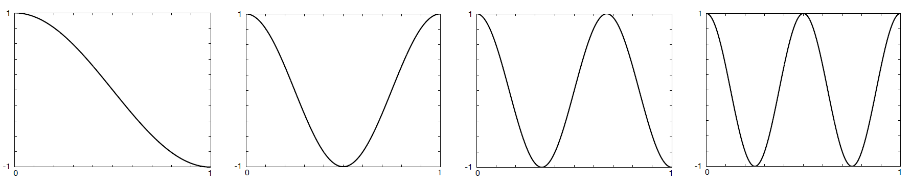
➢Fourier Basis

![\begin{align*}
x_i(s) = \cos(i \pi s), \quad s \in [0,1]
\end{align*}](media/097bec636b.png)
One-dimensional Fourier cosine-basis features for approximating functions over the interval [0, 1].
Linear Function Approximation

Represent state by a feature vector
Feature construction for Linear Methods
➢Polynomials
➢Fourier Basis
➢Coarse Coding
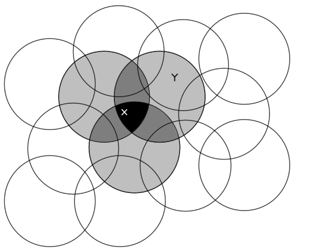
Coarse coding provides large features vector x(s)
Parameter vector w gives a value to each feature.
➢We aggregate multiple states
➢This means the resulting feature vector/agent state is non-Markovian
➢This is the common case when using function approximation
➢Consider whether good solutions exist for given features + function approximation
➢Neural networks tend to be more flexible
Linear Function Approximation

Represent state by a feature vector
Feature construction for Linear Methods
➢Polynomials
➢Fourier Basis
➢Coarse Coding
➢Tile Coding
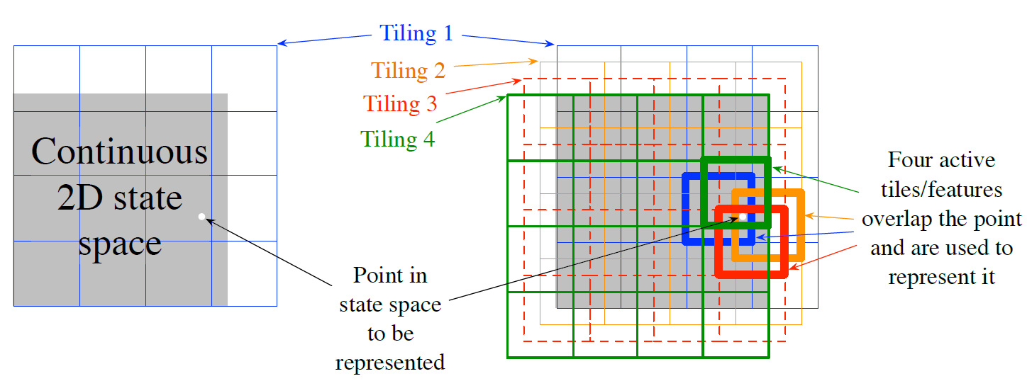
Linear Function Approximation

Represent state by a feature vector
Feature construction for Linear Methods
➢Polynomials
➢Fourier Basis
➢Coarse Coding
➢Tile Coding
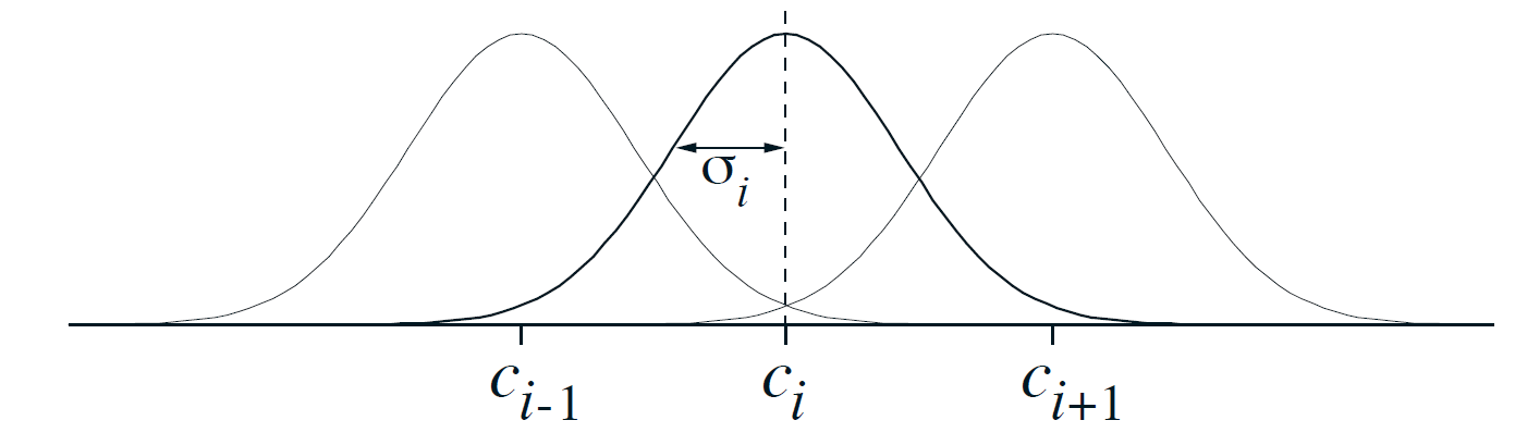
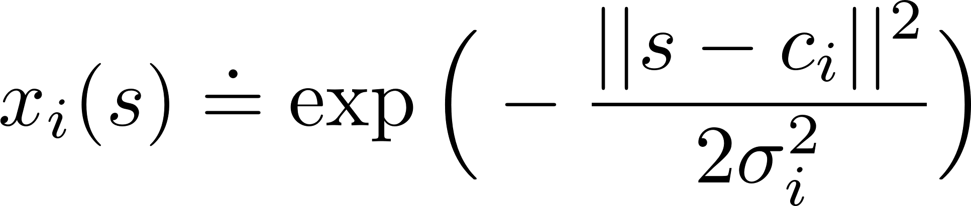
➢Radial Basis Function
(Generalization of coarse coding to continuous-valued features)
Linear Value Function Approximation

![\begin{align*}
= \mathbb{E}_{S \sim d}[(v_{\pi}(S) - \mathbf{w}^T\mathbf{x}(S))^2]
\end{align*}](media/987d8ba5c7.png)
![\begin{align*}
J(\mathbf{w}) = \mathbb{E}_{S \sim d}[(v_{\pi}(S) - v_{\mathbf{w}}(S))^2]
\end{align*}](media/a521b77bc8.png)
Objective function:
Approximate value function by a
linear combination of features
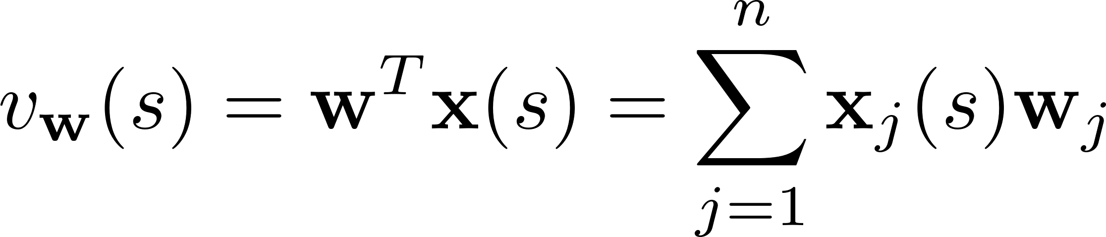
quadratic in w
Stochastic gradient descent
converges on global optimum!
Linear Value Function Approximation
Approximate value function by a
linear combination of features

![\begin{align*}
= \mathbb{E}_{S \sim d}[(v_{\pi}(S) - \mathbf{w}^T\mathbf{x}(S))^2]
\end{align*}](media/987d8ba5c7.png)

![\begin{align*}
J(\mathbf{w}) = \mathbb{E}_{S \sim d}[(v_{\pi}(S) - v_{\mathbf{w}}(S))^2]
\end{align*}](media/a521b77bc8.png)
Objective function:

Stochastic gradient descent:


Update = step-size x prediction error x feature vector

Linear Value Function Approximation
Approximate value function by a
linear combination of features

![\begin{align*}
= \mathbb{E}_{S \sim d}[(v_{\pi}(S) - \mathbf{w}^T\mathbf{x}(S))^2]
\end{align*}](media/987d8ba5c7.png)


![\begin{align*}
J(\mathbf{w}) = \mathbb{E}_{S \sim d}[(v_{\pi}(S) - v_{\mathbf{w}}(S))^2]
\end{align*}](media/a521b77bc8.png)
Objective function:

Stochastic gradient descent:

Update = step-size x prediction error x feature vector
Linear Value Function Approximation
Approximate value function by a
linear combination of features

![\begin{align*}
= \mathbb{E}_{S \sim d}[(v_{\pi}(S) - \mathbf{w}^T\mathbf{x}(S))^2]
\end{align*}](media/987d8ba5c7.png)


![\begin{align*}
J(\mathbf{w}) = \mathbb{E}_{S \sim d}[(v_{\pi}(S) - v_{\mathbf{w}}(S))^2]
\end{align*}](media/a521b77bc8.png)
Objective function:

Stochastic gradient descent:

Update = step-size x prediction error x feature vector

Linear Value Function Approximation for Prediction: MC
Monte-Carlo: is an unbiased sample of true value
Apply “supervised learning” to (online) “training data”:


Linear Monte-Carlo evaluation converges to the global optimum
Even when using non-linear value function approximation it converges
(but perhaps to a local optimum)
Linear Value Function Approximation for Prediction: TD(0)
TD(0): is a biased sample of true value
Apply “supervised learning” to (online) “training data”:

This is akin to a non-stationary regression problem
But it’s a bit different: the target depends on our parameters!

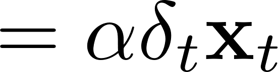
TD-error
Control with value-function approximation
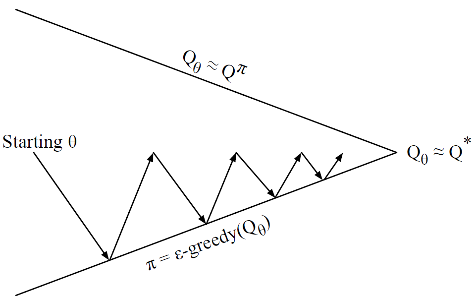
Policy evaluation: Approximate policy evaluation,
Policy improvement: E.g., -greedy policy improvement
Action-Value Function Approximation
Approximate the action-value function
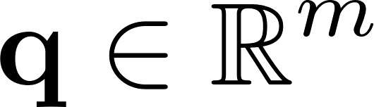
For instance, with linear function approximation with state-action features

Stochastic gradient descent update


Action-Value Function Approximation
Approximate the action-value function
For instance, with linear function approximation with state-action features

Stochastic gradient descent update
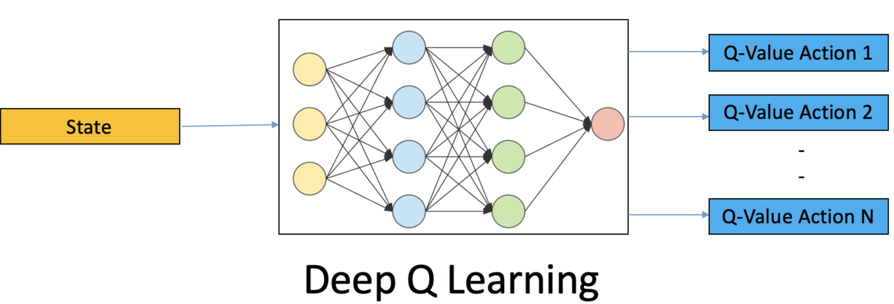


state

Action-Value Function Approximation
Approximate the action-value function
For instance, with linear function approximation with state-action features

Stochastic gradient descent update


state



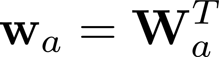
![\begin{align*}
q_{\mathbf{w}}(s,a) = \mathbf{q}_{\mathbf{w}}(s)[a] = \mathbf{x}(s)^T \mathbf{w}_a
\end{align*}](media/9521ca4458.png)


Action-Value Function Approximation
Approximate the action-value function
For instance, with linear function approximation with state-action features

Stochastic gradient descent update


state
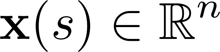


![\begin{align*}
q_{\mathbf{w}}(s,a) = \mathbf{q}_{\mathbf{w}}(s)[a] = \mathbf{x}(s)^T \mathbf{w}_a
\end{align*}](media/9521ca4458.png)


Action-Value Function Approximation
Should we use action-in, or action-out?
Action in:
Action out:

![\begin{align*}
\mathbf{q}_{\mathbf{w}}(s) = \mathbf{W} \mathbf{x}(s) \text{ such that } q_{\mathbf{w}}(s,a) = \mathbf{q}_{\mathbf{w}}(s)[a]
\end{align*}](media/75597c2cf2.png)
One reuses the same weights, the other the same features
Unclear which is better in general
If we want to use continuous actions, action-in is easier (later lecture on actor-critic)
For (small) discrete action spaces, action-out is common (e.g., DQN)

Convergence Questions
➢When do incremental prediction algorithms converge?
➢When using bootstrapping (i.e. TD)?
➢When using (e.g., linear) value function approximation?
➢When using off-policy learning?
➢Ideally, we would like algorithms that converge in all cases
➢Alternatively, we want to understand when algorithms do, or do not, converge
Example of divergence
x = 1
x = 2
r = 0
v = w
v = 2w



Let’s use TD only on this transition.

Example of divergence
x = 1
x = 2
r = 0
v = w
v = 2w
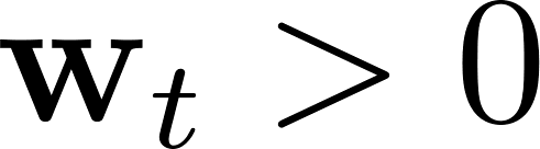
Algorithms that combine
➢bootstrapping
➢off-policy learning
➢function approximation
… may diverge
Deadly triad
Convergence of Prediction Algorithms
On/Off-Policy | Algorithm | Table Lookup | Linear | Non-Linear |
On-Policy | MC | |||
TD | ||||
Off-Policy | MC | |||
TD |
Deadly triad
Bootstrapping
Off-policy
Function Approximation
Convergence of Control Algorithms
➢Tabular control learning algorithms (e.g., Q-learning) can be extended to FA
(e.g., Deep Q Network — DQN)
➢The theory of control with function approximation is not fully developed
➢Tracking is often preferred to convergence
(I.e., continually adapting the policy instead of converging to a fixed policy)
Experience Replay
Batch methods seek to find the best fitting value function for a given set of past experience (“training data")
Given experience consisting of trajectories of experience

1. Sample transition(s), e.g., for
2. Apply stochastic gradient descent update

3. Can re-use old data
Repeat
This is a form of batch learning
Beware: the data may be off-policy if the policy changes!
Take home message
•For MDPs with large state and action spaces, VFA can be used.
•There are different classes of VFA: tabular, linear, and non-linear.
•Stochastic gradient descent can be used to approximate the true value function.
•Divergence can occur when combining:
•Bootstrapping
•Off-policy learning
•Function approximation
Take home message
•Further studying:
•Sections 9.1, 9.2, 9.3, 9.4, 9.5, 9.7, 10.1, 11.3 from the book Reinforcement Learning: An
Introduction
•Short notes: https://people.stfx.ca/jdelamer/courses/csci-531/lectures/rl/approximate-
solutions/on-policy-prediction.html
•Video (UCL x DeepMind)
•Lectures 7:
https://www.youtube.com/watch?v=ook46h2Jfb4&list=PLqYmG7hTraZCRwoyGxvQkqVrZgDQi4m-
5&index=7&t=13s
•Next lecture:
•Policy Gradient and Actor-Critic