

Reinforcement Learning · Lecture 7
Policy Gradients and Actor Critics
Rafael Fernandes Cunha
Today’s topics
1.Recap on function approximation
2.The Policy Gradient Theorem
3.Monte-Carlo Policy Gradient (REINFORCE)
4.Actor-Critic Algorithms
2
1.Explain the advantages of stochastic policies
2.Understand the Policy Gradient Theorem
3.Explain the REINFORCE algorithm
4.Explain the Actor-Critic algorithms
Learning outcomes
Value function approximation
Solution for large MDPs
Estimate value function with function approximation.


Update parameter w
Using MC or TD learning.
Generalize to unseen states
Monte Carlo:
TD(0):
TD():
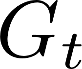


Approximate Values By Stochastic Gradient Descent

![\begin{align*}
J(\mathbf{w}) = \mathbb{E}_{S \sim d}[(v_{\pi}(S) - v_{\mathbf{w}}(S))^2]
\end{align*}](media/a521b77bc8.png)
Goal: Learn the state-value function


Stochastic Gradient Descent
How do we approximate the true
(target) value when sampling?
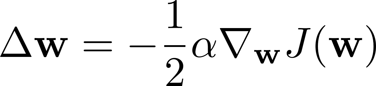
Bootstrapping methods include
only a part of the gradient. We call
them semi-gradient methods.
Linear Function Approximation
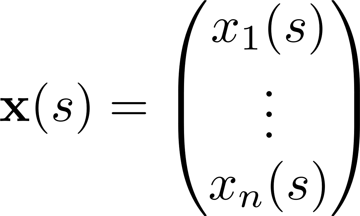
Represent state by a feature vector
Feature construction for Linear Methods
➢Polynomials
➢Fourier Basis
➢Coarse Coding
➢Tile Coding
➢Radial Basis Function
(Generalization of coarse coding to continuous-valued features)
Linear Value Function Approximation for Prediction
Monte-Carlo: is an unbiased sample of true value


TD(0): is a biased sample of true value

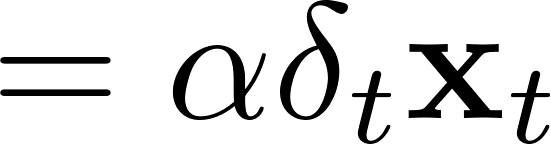

TD-error
Action-Value Function Approximation
SARSA is TD applied to state-action pairs

![\begin{align*}
\mathbf{w}_{t+1} \doteq \mathbf{w}_t + \alpha \Big[{\color{blue}R_{t+1} + \gamma q_{\mathbf{w}_t}(S_{t+1}, A_{t+1})}- q_{\mathbf{w}}(S_t, A_t)\Big] \nabla q_{\mathbf{w}_t}(S_t, A_t)
\end{align*}](media/a47df3cac6.png)
Episodic semi-gradient one-step SARSA
Convergence of Prediction Algorithms
On/Off-Policy | Algorithm | Table Lookup | Linear | Non-Linear |
On-Policy | MC | |||
TD | ||||
Off-Policy | MC | |||
TD |
Deadly triad
Bootstrapping
Off-policy
Function Approximation
General overview
Model-free RL
Monte Carlo
SARSA
q-learning
double q-learning
Expected SARSA
REINFORCE
Actor-Critics
Value-based methods
Policy-based methods
Today’s Lecture
General overview
Model-free RL
Value-based methods
Policy-based methods
Sometimes learning a policy is easier (e.g., “always move forward” is optimal)
Estimate or
Learn a policy
Usually deterministic
Learn a policy
Usually stochastic
Uses some objective function
Learns the policy directly!
Advantages x Disadvantages of Policy-based RL
➢True objective
➢Easy extended to high-dimensional or continuous action spaces
➢Can learn stochastic policies
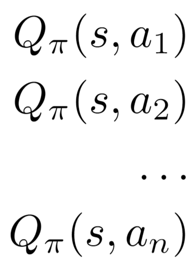
Why do value-based methods
have difficulties to handle this?
![\begin{align*}
Q_{\pi}(s,a_1) \\ Q_{\pi}(s,a_2) \\[1ex] \dots \\[1ex] Q_{\pi}(s,a_n)
\end{align*}](media/ef04c5c5ad.png)
How to take the max of
infinite options of actions?
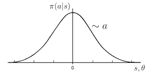
How would a deterministic policy look like?
Advantages
Advantages x Disadvantages of Policy-based RL
➢True objective
➢Easy extended to high-dimensional or continuous action spaces
➢Can learn stochastic policies
➢Sometimes policies are simple while values and models are complex
Advantages
Disadvantages
➢Could get stuck in local optima
➢Obtained knowledge can be specific, does not always generalize well
➢Does not necessarily extract all useful information from the data (when used in isolation)
Benefits of stochastic policies
MDP’s
Fully observable problem
There is always an optimal deterministic policy
The optimal policy may be stochastic
Real World
Not Fully observable problem
Observability
Search Space
Exploration
Search space is smoother for stochastic policies
It is possible to use gradients
Provides some “exploration” during learning
Why?
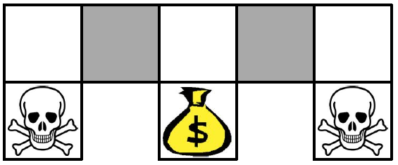
Example: Aliased Grid World

Suppose that you are representing the states by features that only says where are walls.
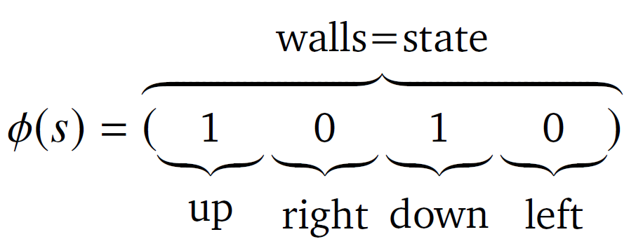
What is the optimal deterministic policy?
Example: Aliased Grid World

Either red or blue policies in grey
states will make the agent get
stuck and never reach the money.
What is the optimal deterministic policy?
Example: Aliased Grid World

What is the optimal stochastic policy?
Move randomly left or right in grey states

Will reach the goal state in a few steps with high probability
Directly learning the policy parameters, we can learn an optimal stochastic policy
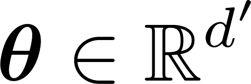
Parameterized Policy
e.g., weights of a
neural network
Restriction: It needs to be
differentiable with respect
to its parameters


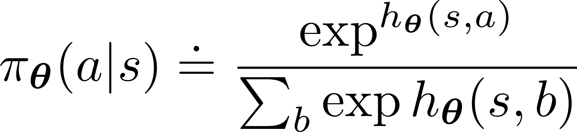
Discrete action space: Actions preferences with soft-max distribution.
Continuous action space: Normal distribution.

Parameterized function approximators.


Parameterized Policy
Learning the policy parameter based on the gradient of some scalar
performance measure with respect to the policy parameter.
e.g., weights of a
neural network
Restriction: It needs to be
differentiable with respect
to its parameters
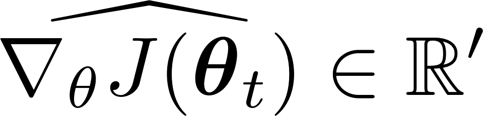


Stochastic estimate whose expectation
approximates the gradient.

How to define the performance measure ?
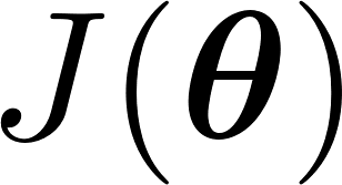
How can we learn ?
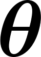

Stochastic gradient ascent in

Performance measure: Episodic return
Goal of RL agent
Find a policy that maximizes the expected return
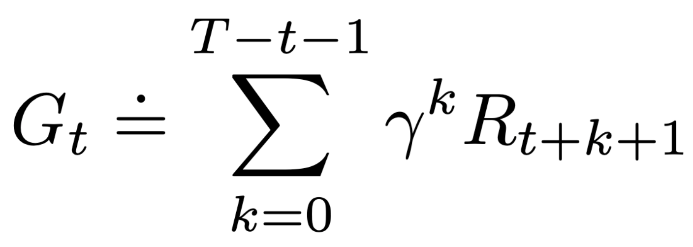

Episodic-return objective

![\begin{align*}
J(\boldsymbol{\theta}) = \mathbb{E}_{\tau \sim p_{\boldsymbol{\theta}}(\tau)}[G(\tau)]
\end{align*}](media/0696ab632b.png)
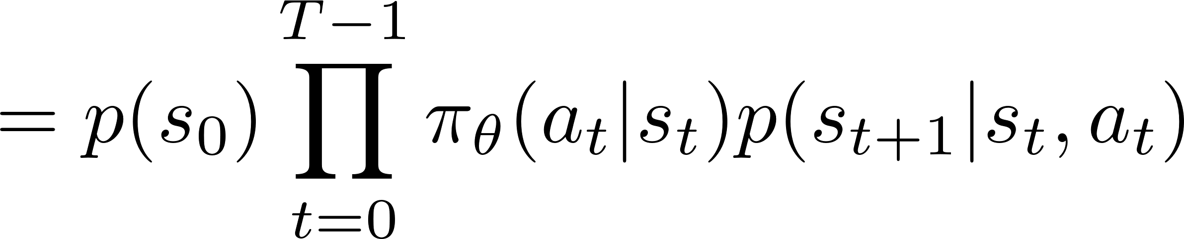
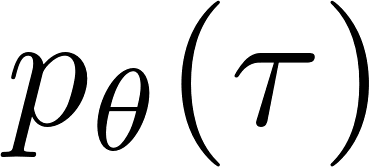
Trajectory

How to compute the probability of a trajectory?
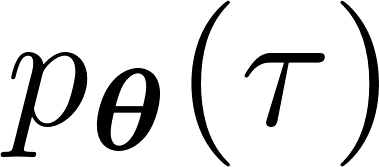
On which functions does it depend?

Return of a trajectory
How to define the performance measure ?

Policy-Gradient derivation
Episodic-return objective
![\begin{align*}
J(\boldsymbol{\theta}) = \mathbb{E}_{\tau \sim p_{\boldsymbol{\theta}}(\tau)}[G(\tau)]
\end{align*}](media/0696ab632b.png)


This objective induces a natural ordering over policies:
![\begin{align*}
\boldsymbol{\theta}^* = \underset{\boldsymbol{\theta}}{\arg \max}\mathbb{E}_{\tau \sim p_{\boldsymbol{\theta}}(\tau)}[G(\tau)]
\end{align*}](media/2f958c01b3.png)
Goal: Find
Policy-Gradient derivation
Episodic-return objective
![\begin{align*}
J(\boldsymbol{\theta}) = \mathbb{E}_{\tau \sim p_{\boldsymbol{\theta}}(\tau)}[G(\tau)]
\end{align*}](media/0696ab632b.png)


![\begin{align*}
\boldsymbol{\theta}^* = \underset{\boldsymbol{\theta}}{\arg \max}\mathbb{E}_{\tau \sim p_{\boldsymbol{\theta}}(\tau)}[G(\tau)]
\end{align*}](media/2f958c01b3.png)
Goal: Find

Stochastic gradient ascent:
Policy-Gradient derivation
Stochastic gradient ascent:

![\begin{align*}
=\nabla_{\boldsymbol{\theta}}\mathbb{E}_{\tau \sim p_{\boldsymbol{\theta}}(\tau)}[G(\tau)]
\end{align*}](media/b881129e66.png)
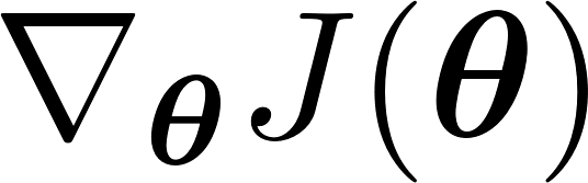
What is the difficulty in computing this expression?
We cannot sample the gradient of an expectation!
Idea: Move the gradient “inside” the expectation and sample the expression!
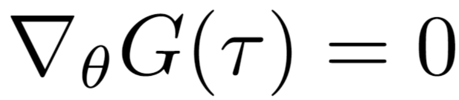
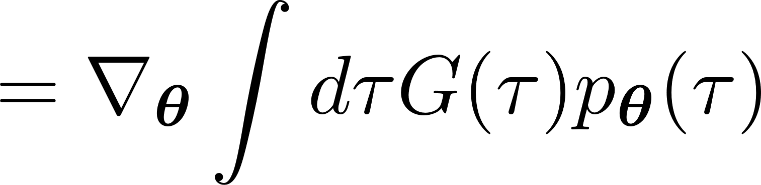
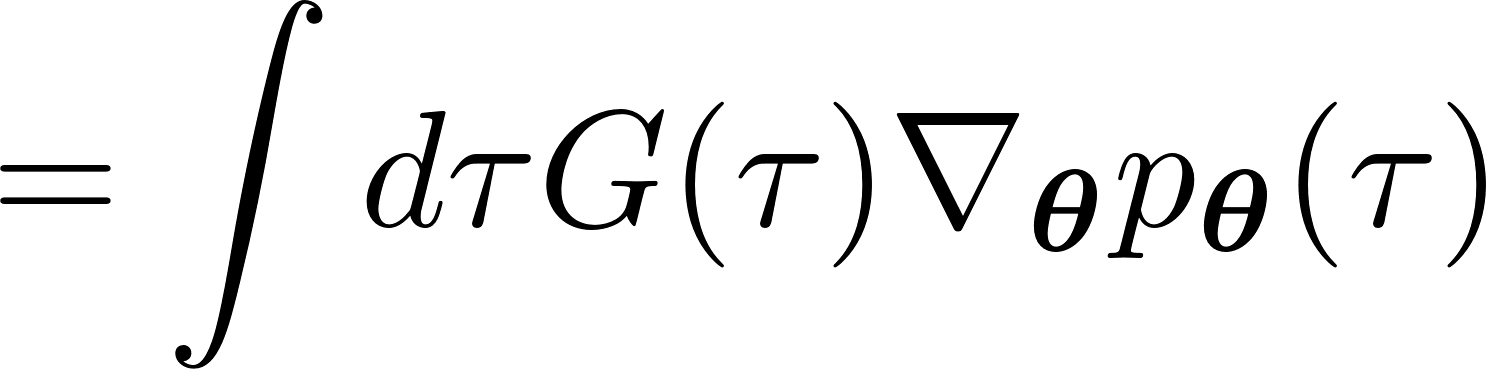
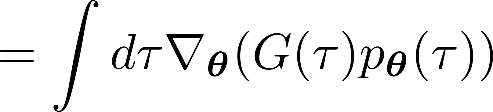
Policy-Gradient derivation
Stochastic gradient ascent:

Definition of expectation
Linearity of the gradient
Chain rule
![\begin{align*}
=\nabla_{\boldsymbol{\theta}}\mathbb{E}_{\tau \sim p_{\boldsymbol{\theta}}(\tau)}[G(\tau)]
\end{align*}](media/b881129e66.png)


Policy-Gradient derivation
Stochastic gradient ascent:
Definition of expectation
Linearity of the gradient
Chain rule



![\begin{align*}
=\nabla_{\boldsymbol{\theta}}\mathbb{E}_{\tau \sim p_{\boldsymbol{\theta}}(\tau)}[G(\tau)]
\end{align*}](media/b881129e66.png)


How to write it in terms of expectation!

![\begin{align*}
=\mathbb{E}_{\tau \sim p_{\boldsymbol{\theta}}(\tau)}[ G(\tau)\nabla_{\boldsymbol{\theta}}p_{\boldsymbol{\theta}}(\tau)]
\end{align*}](media/5412b56721.png)

We are missing this term in our expression!
Policy-Gradient derivation
Stochastic gradient ascent:
Definition of expectation
Linearity of the gradient
Chain rule


![\begin{align*}
=\nabla_{\boldsymbol{\theta}}\mathbb{E}_{\tau \sim p_{\boldsymbol{\theta}}(\tau)}[G(\tau)]
\end{align*}](media/b881129e66.png)


Derivative of a logarithm
Definition of expectation
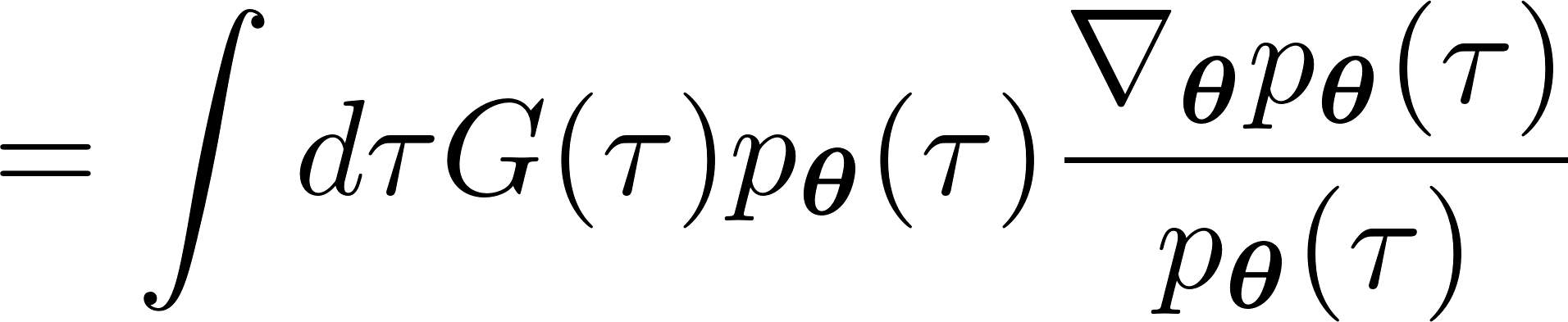

![\begin{align*}
= \mathbb{E}_{\tau \sim p_{\boldsymbol{\theta}}(\tau)}[ G(\tau) \nabla_{\boldsymbol{\theta}} \log(p_{\boldsymbol{\theta}}(\tau))]
\end{align*}](media/ad8d0fa120.png)
Policy-Gradient derivation
Stochastic gradient ascent:


![\begin{align*}
= \mathbb{E}_{\tau \sim p_{\boldsymbol{\theta}}(\tau)}[ G(\tau) \nabla_{\boldsymbol{\theta}} \log(p_{\boldsymbol{\theta}}(\tau))]
\end{align*}](media/ad8d0fa120.png)
Now we can sample this expression!
This product can be converted into a summation by applying a logarithm!
But how to compute this gradient?

?
Policy-Gradient derivation




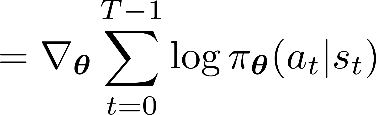


It does not depend on theta!

![\begin{align*}
= \mathbb{E}_{\tau \sim p_{\boldsymbol{\theta}}(\tau)}[ G(\tau) \nabla_{\boldsymbol{\theta}} \log(p_{\boldsymbol{\theta}}(\tau))]
\end{align*}](media/ad8d0fa120.png)
Policy-Gradient derivation


This probability depends on the policy
and the transition function.
This term only depends on the policy!

![\begin{align*}
= \mathbb{E}_{\tau \sim p_{\boldsymbol{\theta}}(\tau)}[ G(\tau) \nabla_{\boldsymbol{\theta}} \log(p_{\boldsymbol{\theta}}(\tau))]
\end{align*}](media/ad8d0fa120.png)
Policy-Gradient derivation


![\begin{align*}
= \mathbb{E}_{\tau \sim p_{\boldsymbol{\theta}}(\tau)}[ G(\tau) \nabla_{\boldsymbol{\theta}} \log(p_{\boldsymbol{\theta}}(\tau))]
\end{align*}](media/ad8d0fa120.png)
![\begin{align*}
= \mathbb{E}_{\tau \sim p_{\boldsymbol{\theta}}(\tau)}[ G(\tau) \nabla_{\boldsymbol{\theta}}\sum_{t=0}^{T-1}\log \pi_{\boldsymbol{\theta}}(a_t|s_t) ]
\end{align*}](media/3eff878b89.png)
![\begin{align*}
= \mathbb{E}_{\tau \sim p_{\boldsymbol{\theta}}(\tau)}\Big[ \Big( \sum_{t=0}^{T-1} \nabla_{\boldsymbol{\theta}}\log \pi_{\boldsymbol{\theta}}(a_t|s_t)\Big) G(\tau)\Big]
\end{align*}](media/78b3d4bcc2.png)
![\begin{align*}
= \mathbb{E}_{\tau \sim p_{\boldsymbol{\theta}}(\tau)}\Big[ \Big( \sum_{t=0}^{T-1} \nabla_{\boldsymbol{\theta}}\log \pi_{\boldsymbol{\theta}}(a_t|s_t)\Big)\Big( \sum_{t=0}^{T-1}r(s_t, a_t) \Big)\Big]
\end{align*}](media/f9405943ca.png)
Let’s sample this expression!

Policy-Gradient Theorem


![\begin{align*}
\boldsymbol{\theta}^* = \underset{\boldsymbol{\theta}}{\arg \max}\mathbb{E}_{\tau \sim p_{\boldsymbol{\theta}}(\tau)}[G(\tau)]
\end{align*}](media/2f958c01b3.png)
Goal: Find

The update is
directly proportional to the return of the trajectory
inversely proportional to the policy
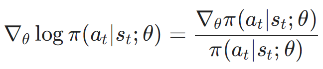
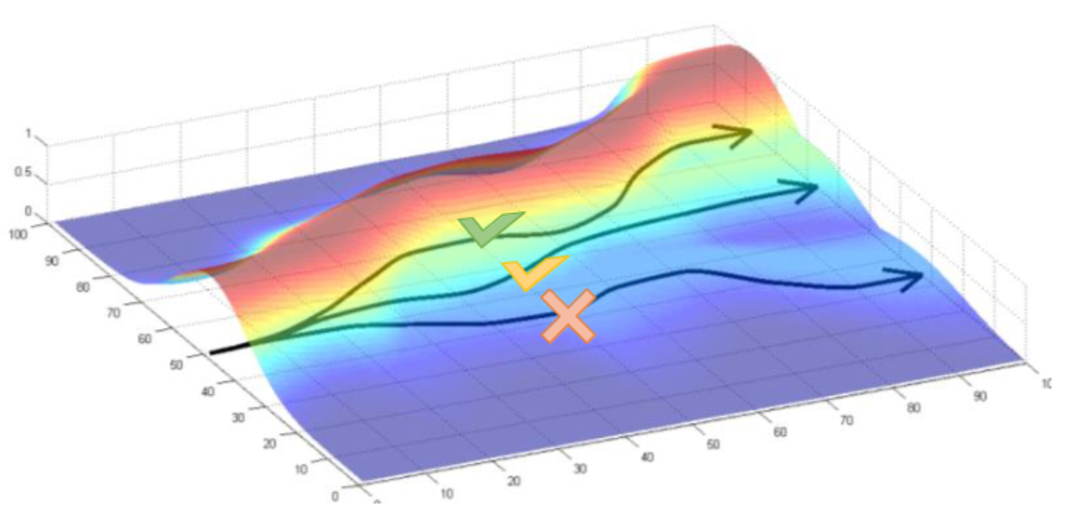
The gradient
rises the log probabilities of the good trajectories
lowers the log probabilities of the bad trajectories
REINFORCE
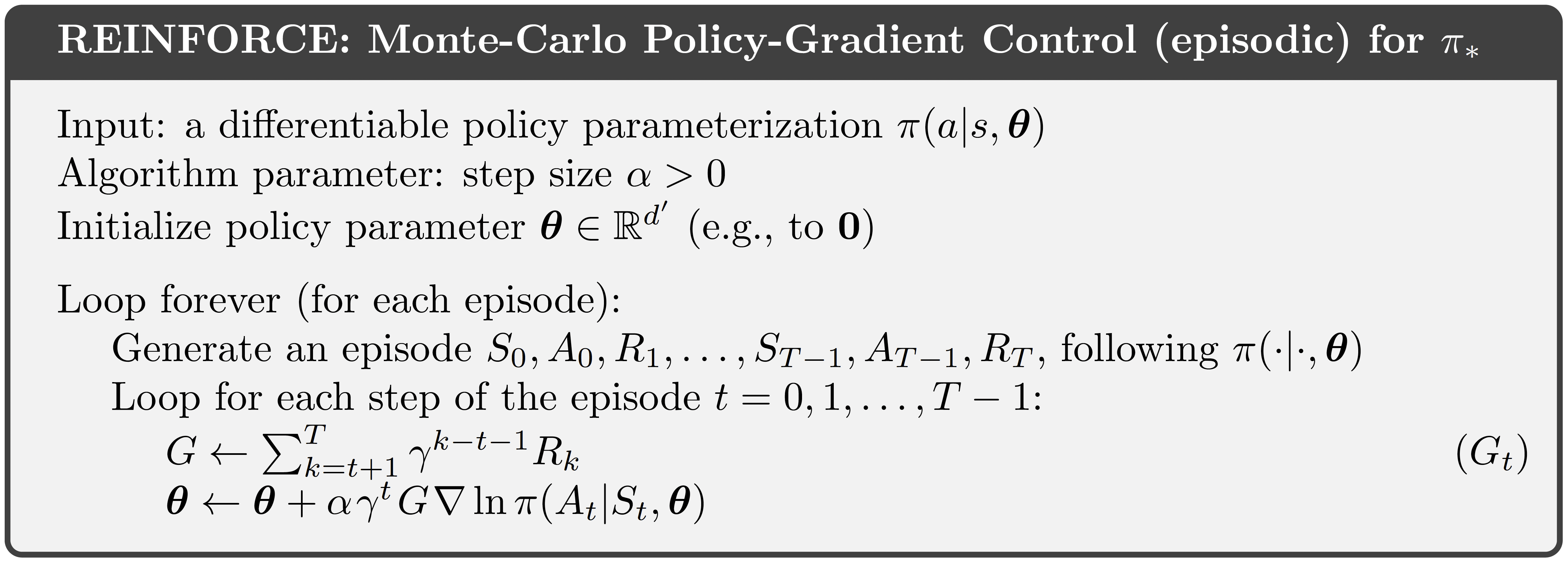
Variance problem on REINFORCE
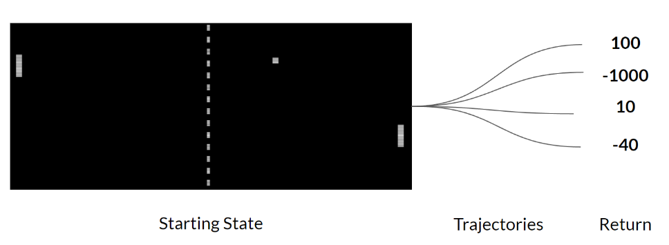
The REINFORCE algorithm is based on the return of an episode!
High variance in the return
Actions have randomness because they are
sampled from a probability distribution.
The starting state may vary per episode.
The environment transition function may be stochastic.
Reducing the variance: Causality



Causality: policy at time cannot affect reward at time when
Reducing the variance: Causality
The action-value function!
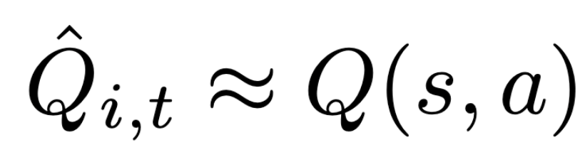


Causality: policy at time cannot affect reward at time when
reward “to-go”
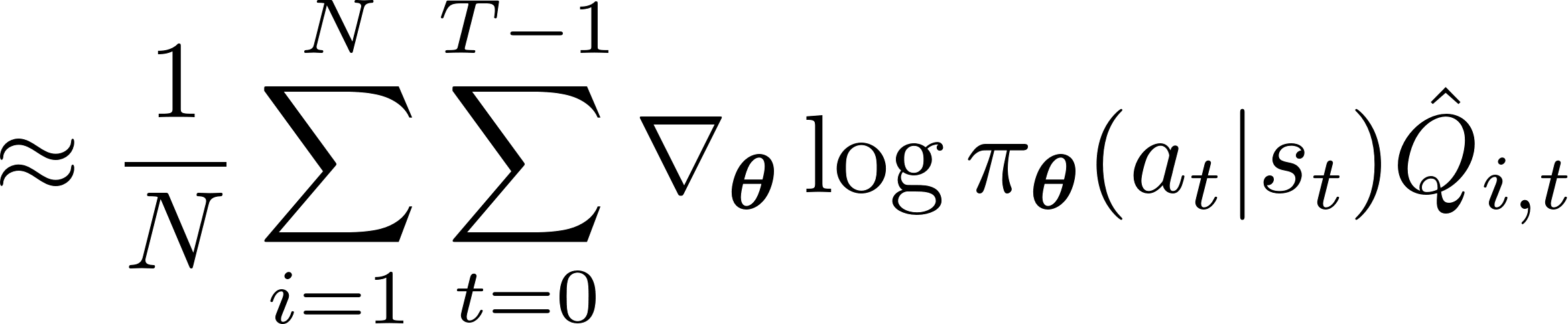

Which function has a similar definition?
Reducing the variance: Baseline
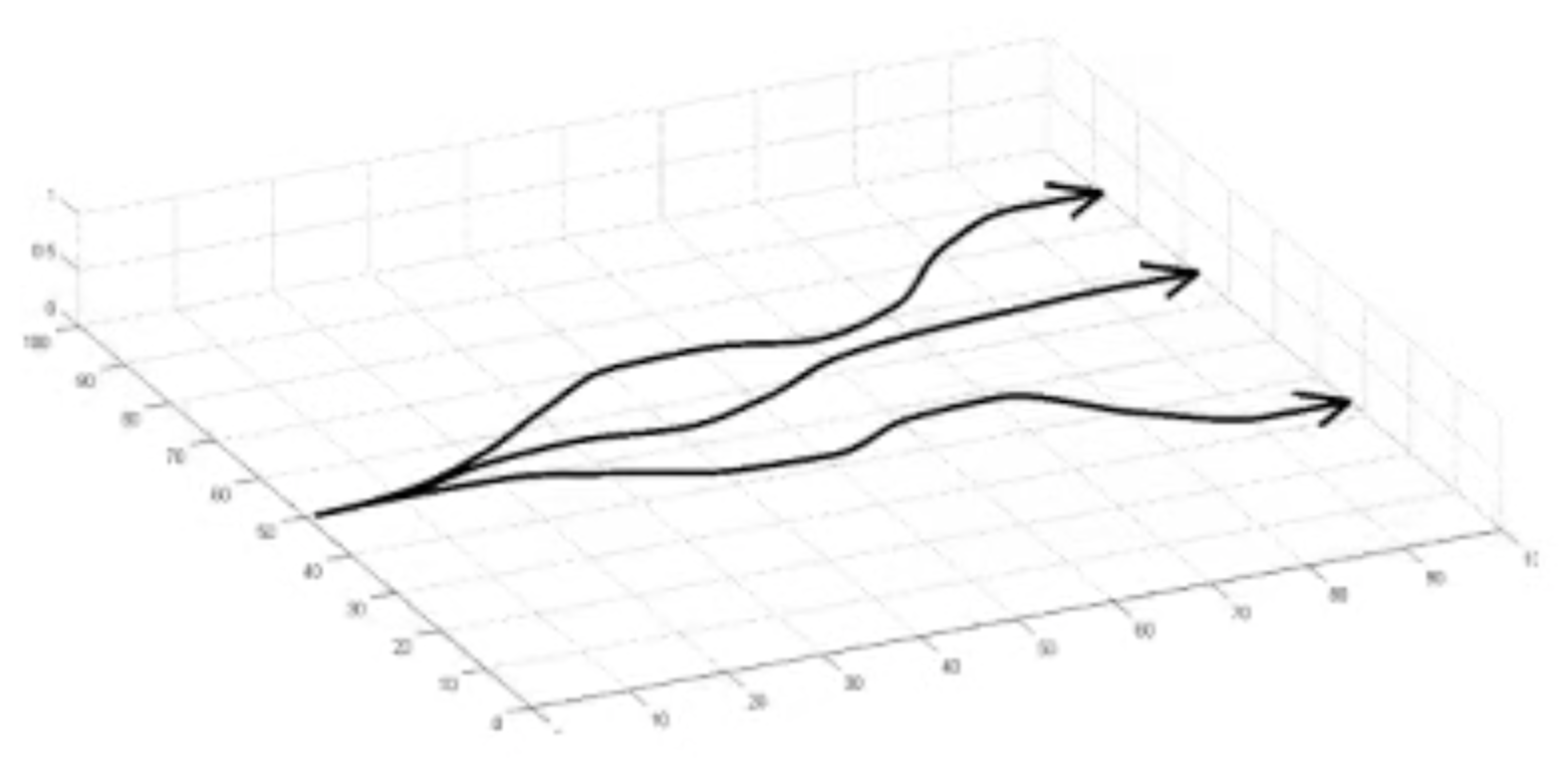

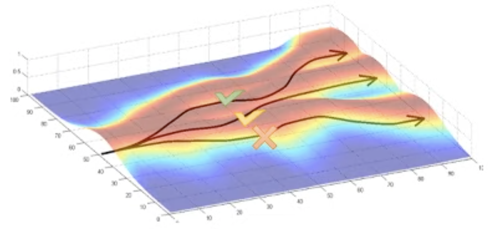
Without Baseline
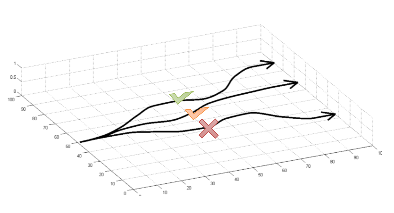
With Baseline
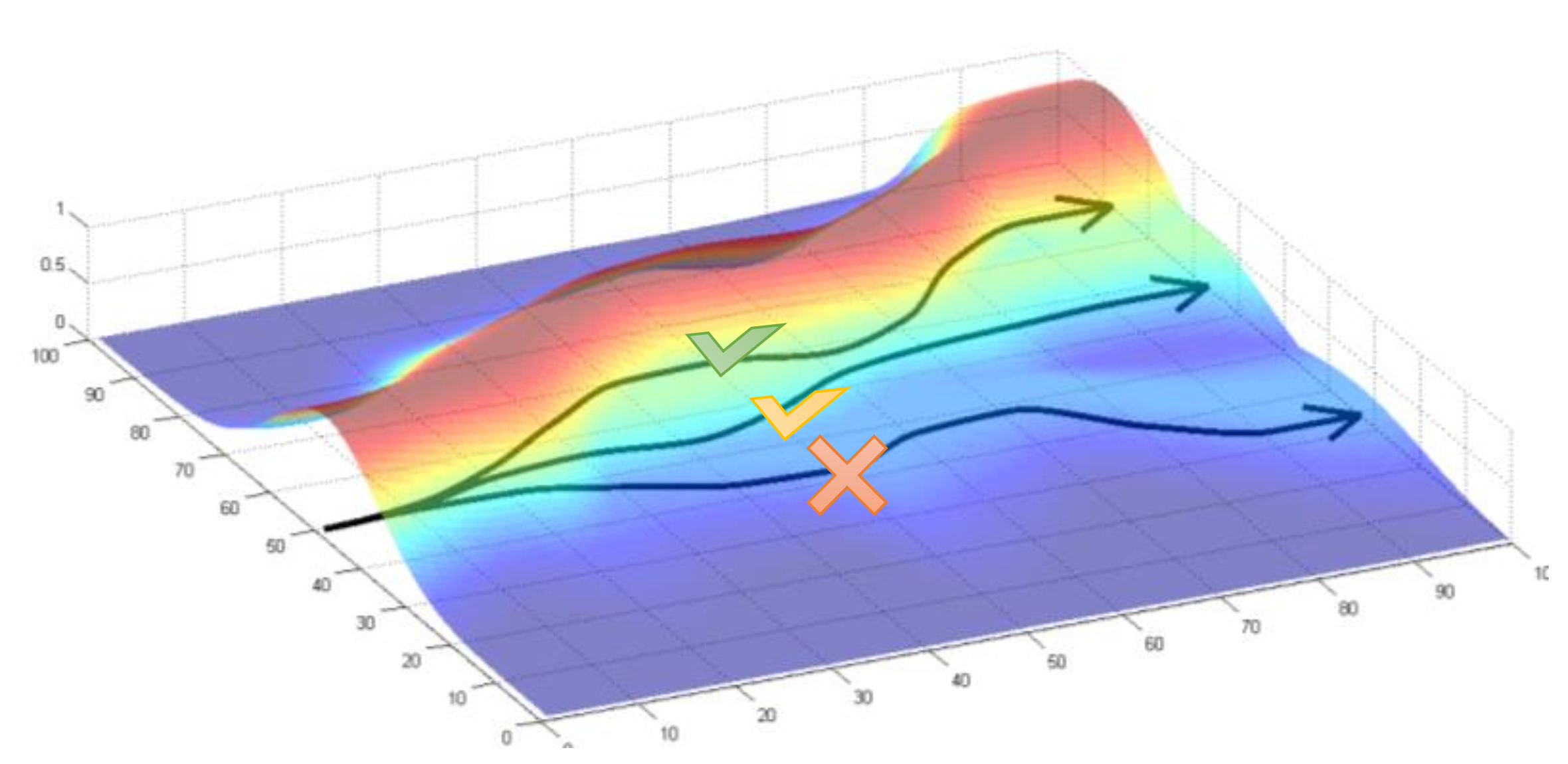
All positive
Subtracting a baseline independent from the action.

![\begin{align*}
\nabla_\theta J(\theta) = \mathbb{E}_{\tau\sim p_\theta(\tau)}\Big[\nabla_\theta \log p_\theta(\tau)(G_t(\tau) - b)\Big]
\end{align*}](media/47ad4625fb.png)
Example: Average return (not the best baseline)
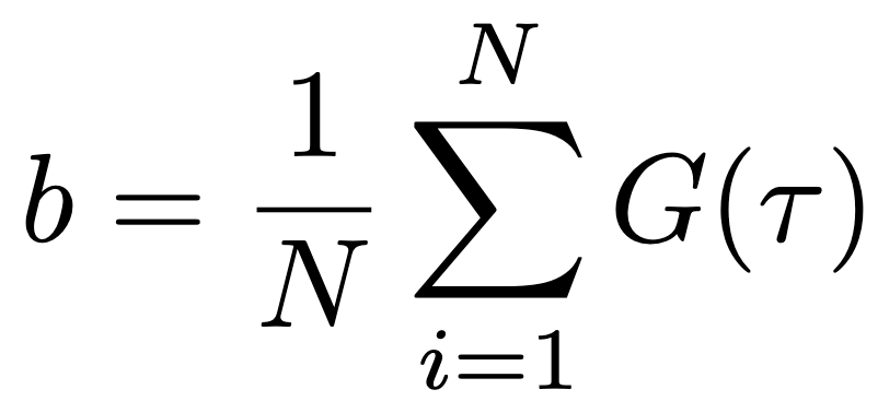
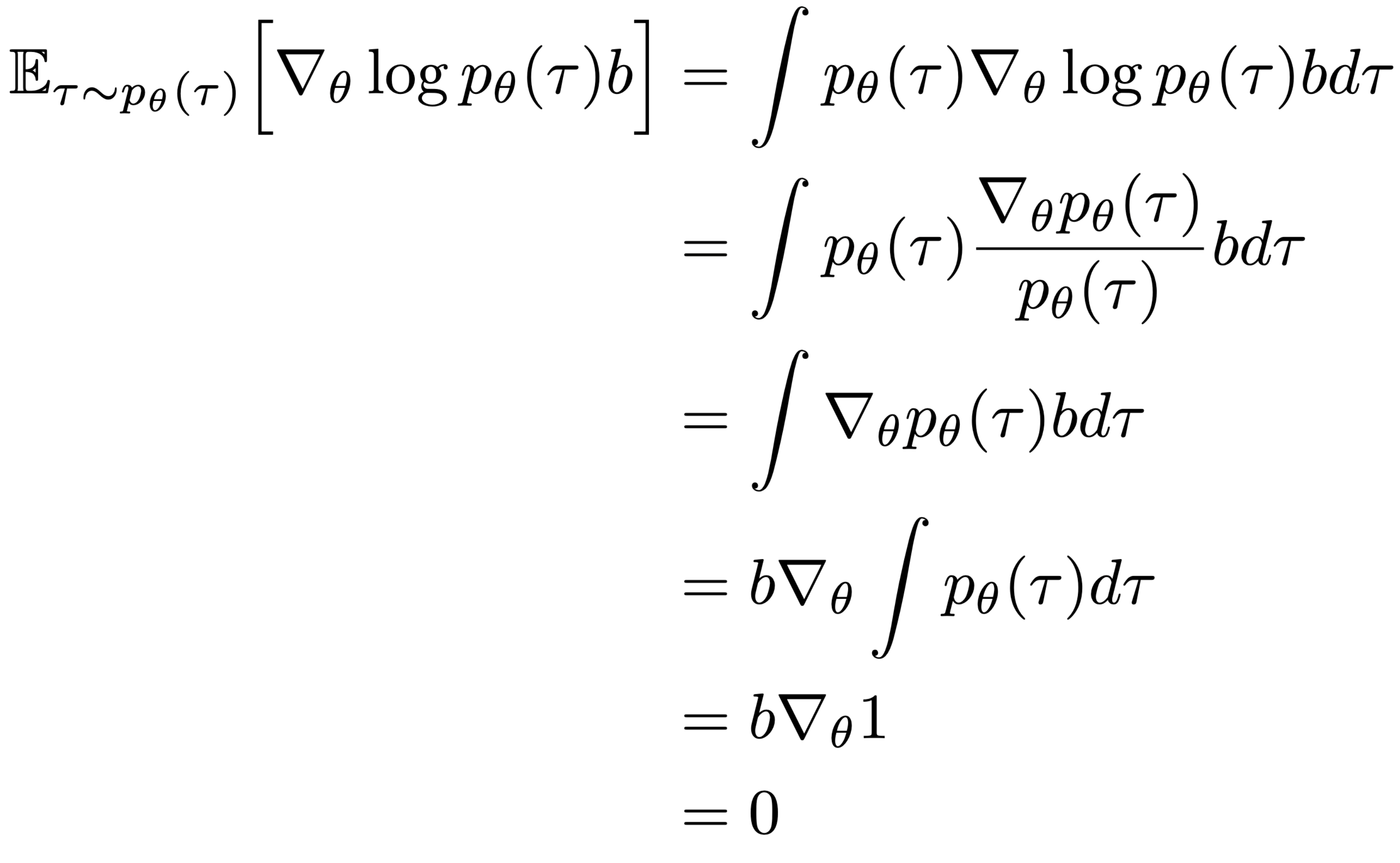
Why the baseline does not introduce bias in the gradient?
Reducing the variance: Baseline
![\begin{align*}
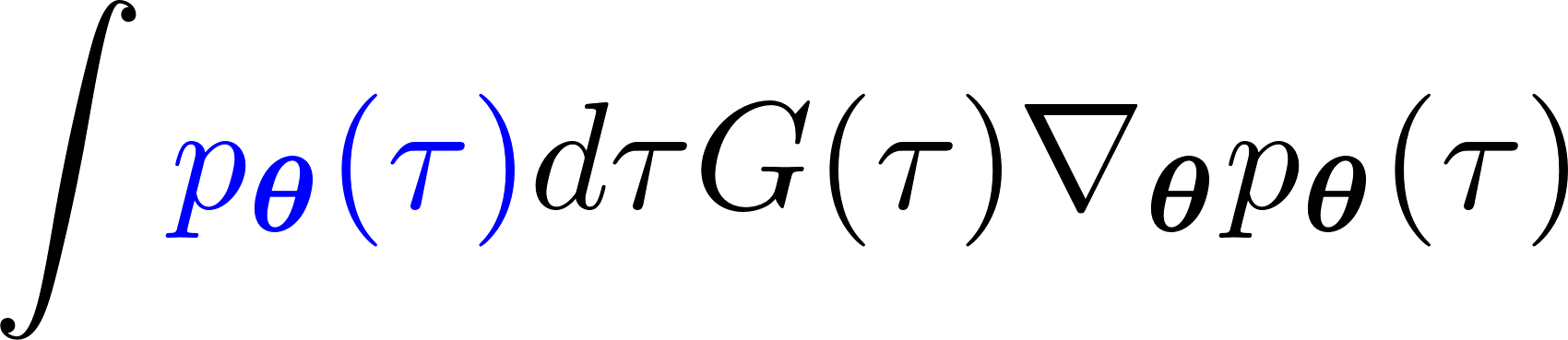
\mathbb{E}_{\tau \sim p_\theta(\tau)} \Big[ \nabla_\theta \log p_\theta(\tau) b \Big] &= \int p_\theta(\tau) \nabla_\theta \log p_\theta(\tau) b d\tau \\ &= \int p_\theta(\tau) \frac{\nabla_\theta p_\theta(\tau)}{p_\theta(\tau)} b d\tau \\ &= \int \nabla_\theta p_\theta(\tau) b d\tau \\ &= b \nabla_\theta \int p_\theta(\tau) d\tau \\ &= b \nabla_\theta 1 \\ &= 0
\end{align*}](media/d79a2e41a8.png)
Subtracting a baseline is unbiased in expectation
![\begin{align*}
\mathbb{E}_{\tau \sim p_\theta(\tau)} \Big[ \nabla_\theta \log p_\theta(\tau) b \Big] &= \int p_\theta(\tau) \nabla_\theta \log p_\theta(\tau) b d\tau \\ &= \int p_\theta(\tau) \frac{\nabla_\theta p_\theta(\tau)}{p_\theta(\tau)} b d\tau \\ &= \int \nabla_\theta p_\theta(\tau) b d\tau \\ &= b \nabla_\theta \int p_\theta(\tau) d\tau \\ &= b \nabla_\theta 1 \\ &= 0
\end{align*}](media/d79a2e41a8.png)
![\begin{align*}
\mathbb{E}_{\tau \sim p_\theta(\tau)} \Big[ \nabla_\theta \log p_\theta(\tau) b \Big] &= \int p_\theta(\tau) \nabla_\theta \log p_\theta(\tau) b d\tau \\ &= \int p_\theta(\tau) \frac{\nabla_\theta p_\theta(\tau)}{p_\theta(\tau)} b d\tau \\ &= \int \nabla_\theta p_\theta(\tau) b d\tau \\ &= b \nabla_\theta \int p_\theta(\tau) d\tau \\ &= b \nabla_\theta 1 \\ &= 0
\end{align*}](media/d79a2e41a8.png)
![\begin{align*}
\mathbb{E}_{\tau \sim p_\theta(\tau)} \Big[ \nabla_\theta \log p_\theta(\tau) b \Big] &= \int p_\theta(\tau) \nabla_\theta \log p_\theta(\tau) b d\tau \\ &= \int p_\theta(\tau) \frac{\nabla_\theta p_\theta(\tau)}{p_\theta(\tau)} b d\tau \\ &= \int \nabla_\theta p_\theta(\tau) b d\tau \\ &= b \nabla_\theta \int p_\theta(\tau) d\tau \\ &= b \nabla_\theta 1 \\ &= 0
\end{align*}](media/d79a2e41a8.png)
![\begin{align*}
\mathbb{E}_{\tau \sim p_\theta(\tau)} \Big[ \nabla_\theta \log p_\theta(\tau) b \Big] &= \int p_\theta(\tau) \nabla_\theta \log p_\theta(\tau) b d\tau \\ &= \int p_\theta(\tau) \frac{\nabla_\theta p_\theta(\tau)}{p_\theta(\tau)} b d\tau \\ &= \int \nabla_\theta p_\theta(\tau) b d\tau \\ &= b \nabla_\theta \int p_\theta(\tau) d\tau \\ &= b \nabla_\theta 1 \\ &= 0
\end{align*}](media/d79a2e41a8.png)
![\begin{align*}
\mathbb{E}_{\tau \sim p_\theta(\tau)} \Big[ \nabla_\theta \log p_\theta(\tau) b \Big] &= \int p_\theta(\tau) \nabla_\theta \log p_\theta(\tau) b d\tau \\ &= \int p_\theta(\tau) \frac{\nabla_\theta p_\theta(\tau)}{p_\theta(\tau)} b d\tau \\ &= \int \nabla_\theta p_\theta(\tau) b d\tau \\ &= b \nabla_\theta \int p_\theta(\tau) d\tau \\ &= b \nabla_\theta 1 \\ &= 0
\end{align*}](media/d79a2e41a8.png)
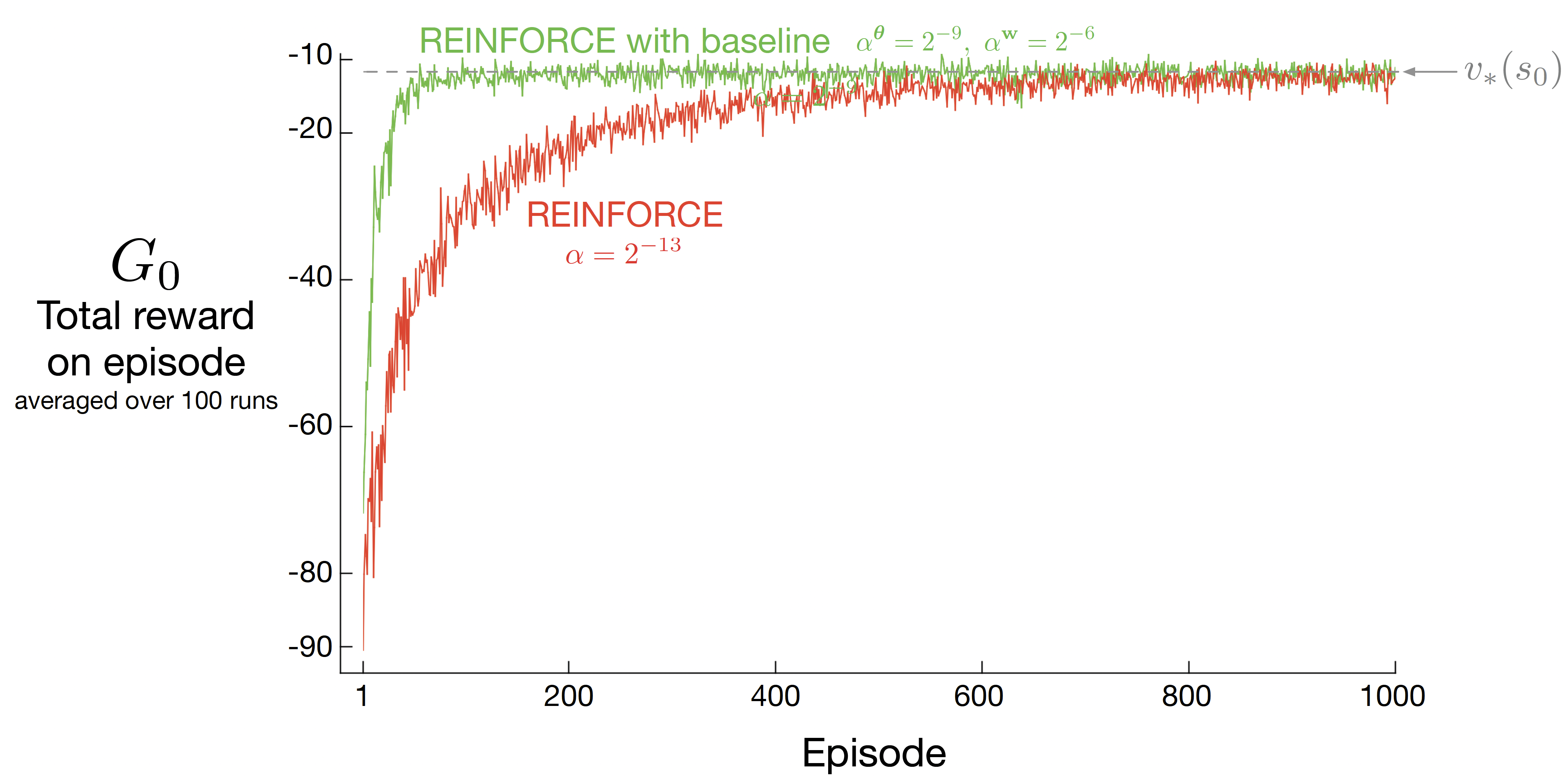
REINFORCE with baseline
![\begin{align*}
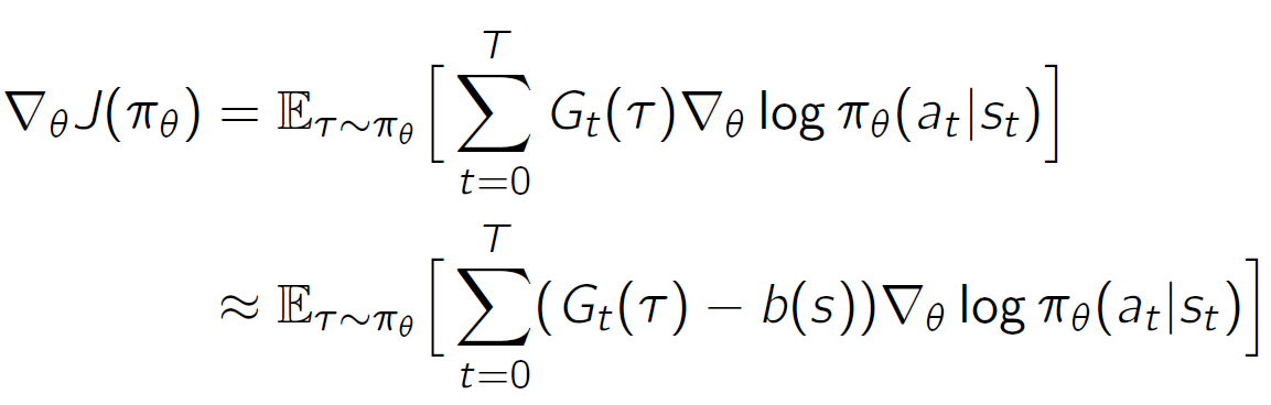
\nabla_\theta J(\pi_\theta) &= \mathbb{E}_{\tau\sim\pi_\theta}\left[\,\sum_{t=0}^{T} G_t(\tau)\nabla_\theta \log \pi_\theta(a_t|s_t)\right] \\ &\approx \mathbb{E}_{\tau\sim\pi_\theta}\left[\,\sum_{t=0}^{T}(\,G_t(\tau) - b(s))\nabla_\theta \log \pi_\theta(a_t|s_t)\right]
\end{align*}](media/7ae5f02bdb.png)
![\begin{align*}
\nabla_\theta J(\pi_\theta) &= \mathbb{E}_{\tau\sim\pi_\theta}\left[\,\sum_{t=0}^{T} G_t(\tau)\nabla_\theta \log \pi_\theta(a_t|s_t)\right] \\ &\approx \mathbb{E}_{\tau\sim\pi_\theta}\left[\,\sum_{t=0}^{T}(\,G_t(\tau) - b(s))\nabla_\theta \log \pi_\theta(a_t|s_t)\right]
\end{align*}](media/7ae5f02bdb.png)
If is , this choice of baselines motivates the Actor-Critic family of algorithms.
Value function parameterized by
Learn the value function via:
MC -> REINFORCE with baseline
TD-learning -> Actor-Critic
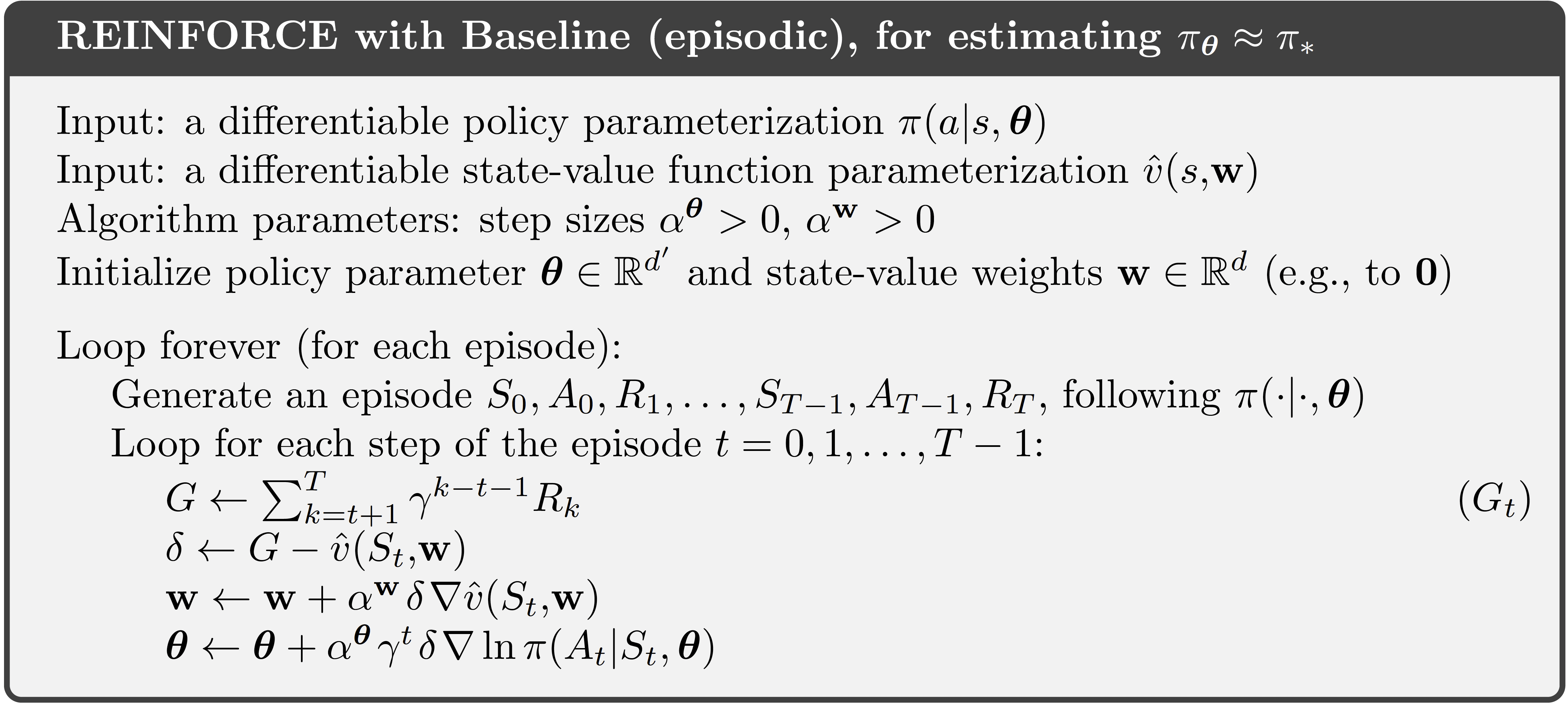
REINFORCE with baseline
Baseline

REINFORCE with baseline
Two learning rates
Actor-Critic algorithms
6
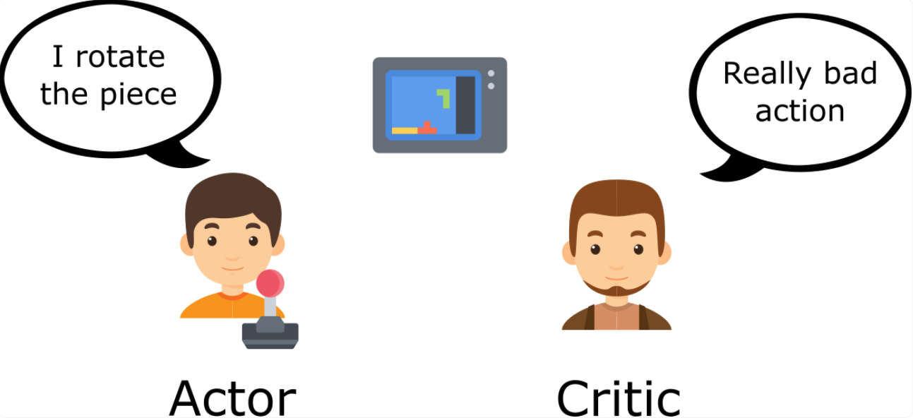
A policy that controls
how our agent acts.
A value function that
measures how good
the action taken is.
Value-Based
Policy-Based
DQN
REINFORCE
Actor-Critic
A2C
Critic
Actor
Actor-Critic algorithms

6
A policy that controls
how our agent acts.
A value function that
measures how good
the action taken is.

Learn two function approximations!
Value-Based
Policy-Based
DQN
REINFORCE
Actor-Critic
A2C
Critic
Actor
Actor-Critic algorithms

6
A policy that controls
how our agent acts.
A value function that
measures how good
the action taken is.


Value-Based
Policy-Based
DQN
REINFORCE
Actor-Critic
A2C
Critic
Actor
Actor-Critic algorithms

6
A policy that controls
how our agent acts.
A value function that
measures how good
the action taken is.
![\begin{align*}
V^{\pi}(s) = \underset{\tau\sim\pi}{\mathrm{E}}\,\left[R(\tau)\,|s_0 = s\right]
\end{align*}](media/e36beaae4f.png)
![\begin{align*}
Q^{\pi}(s,a) = \underset{\tau\sim\pi}{\mathrm{E}}\,\left[R(\tau)\,|s_0 = s, a_0 = a\right]
\end{align*}](media/3021741fed.png)
Value-Based
Policy-Based
DQN
REINFORCE
Actor-Critic
A2C
Critic
Actor
Advantage function

Case 1
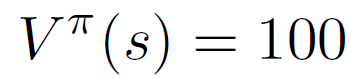


Case 2
Inform the relative improvement caused by action a.

Advantage function!
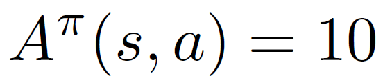

Same Value!
7

CRITIC

Policy gradient step
Direction of the steepest increase
of the (log) probability of
selecting action from state
Return
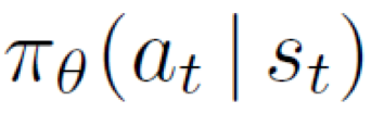
Learns parametrized policy .
8

REINFORCE

Policy gradient step
Return
8

REINFORCE
The entire episode must
finish. High variance.
Learns parametrized policy .

Policy gradient step
Return
8

REINFORCE
Can we use something better?
Learns parametrized policy .

Policy gradient step
Return
8

REINFORCE
Estimate the relative improvement of
action at state . Low variance.

![\begin{align*}
\textit{Actor-Critic:}\quad \nabla_\theta J(\pi_\theta) &= \mathbb{E}_t\big[A_t^{\pi}\nabla_\theta \log \pi_\theta(a_t \mid s_t)\big] \\ \textit{REINFORCE:}\quad \nabla_\theta J(\pi_\theta) &= \mathbb{E}_t\big[R_t(\tau)\nabla_\theta \log \pi_\theta(a_t \mid s_t)\big]
\end{align*}](media/074b1ed676.png)
A2C
Advantage
Learns parametrized policy .
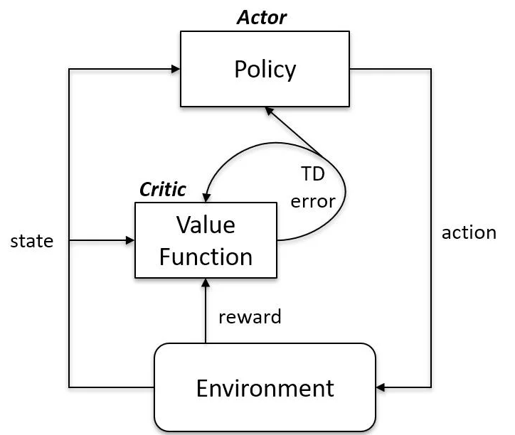
Block Diagram of A2C algorithm


Time Difference (TD) error
Recall the advantage function
Mnih, Volodymyr, et al. "Asynchronous methods for deep reinforcement learning." International conference on machine learning. PMLR, 2016.
9
Agent
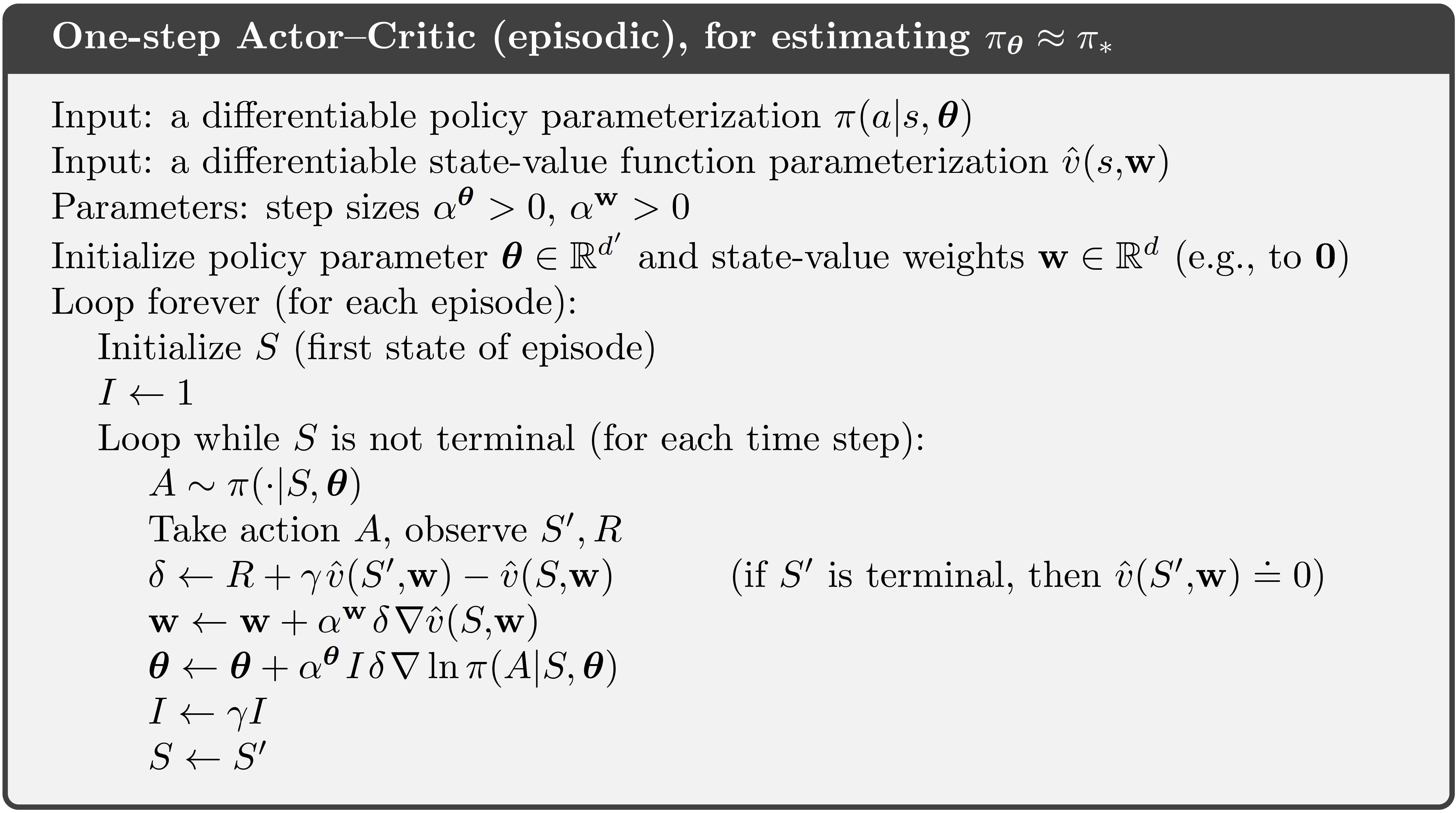
TD-error calculation

Update Critic

Update Actor
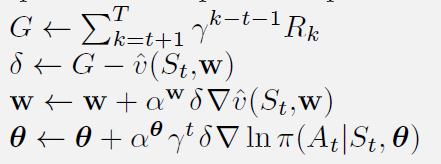

REINFORCE with baseline


Policy gradient algorithms (REINFORCE)
•Suitable for continuous state and action space.
•High variance.


Value based algorithms
•Not suitable for continuous action space.
Summary on policy gradient algorithms
Actor-Critic algorithm
•Suitable for continuous state and action space.
•Low variance.


10
Taxonomy of Deep
RL algorithms
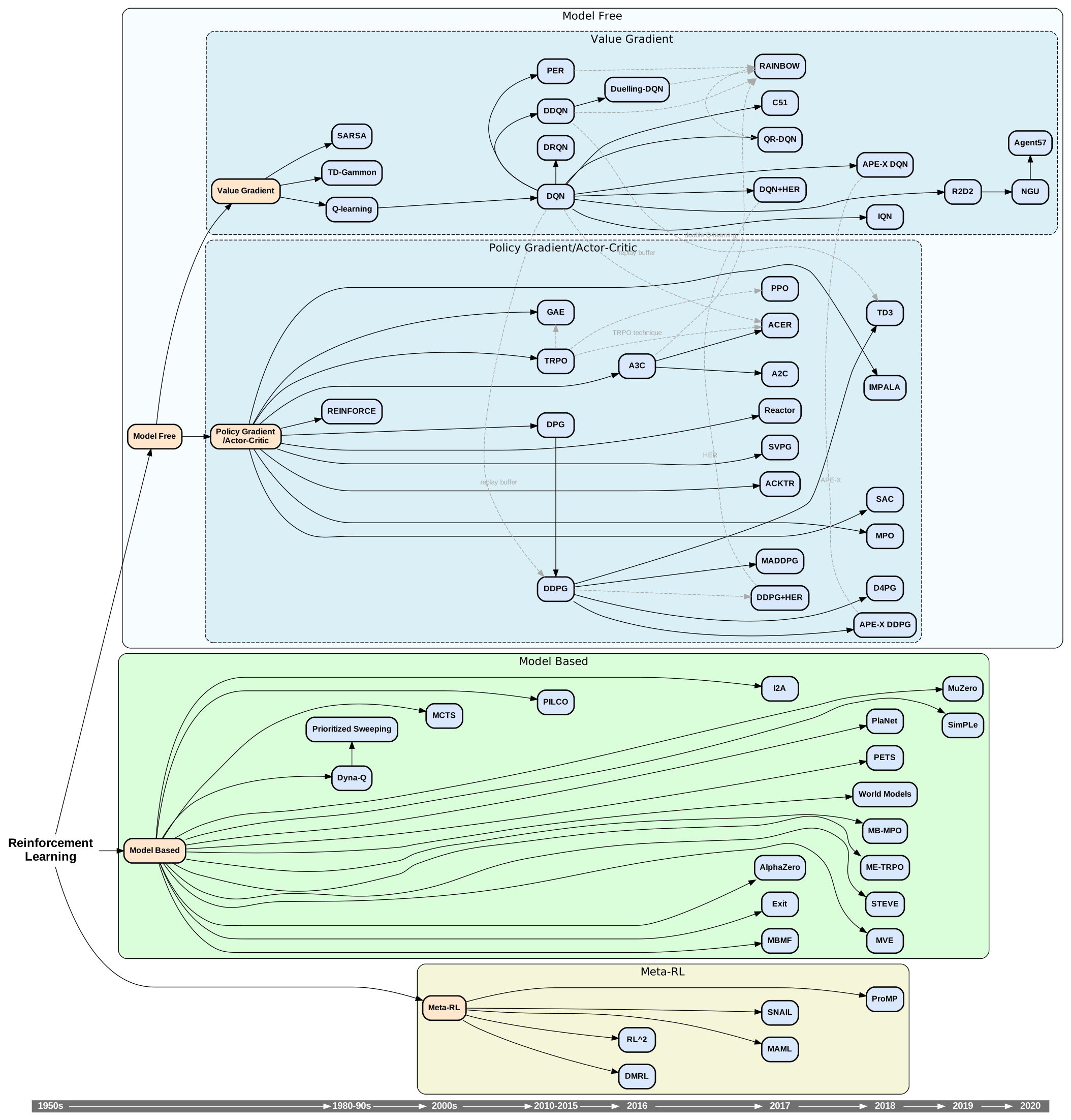
Take home message
•Policy gradient algorithms learn the policy directly
•It is possible to learn stochastic policies
•Suitable for continuous action space problems
•Choosing as baseline introduce actor-critic algorithms
•Actor-critic algorithms use policy gradients and value functions
•Actor-critic algorithms reduce the variance problems of REINFORCE
Take home message
•Further studying:
•Chapter 13– Reinforcement Learning: An introduction
•Short notes: https://people.stfx.ca/jdelamer/courses/csci-531/lectures/rl/policy-gradient/policy-gradient-
methods.html
•Video (UCL x DeepMind)
•Lectures 9:
https://www.youtube.com/watch?v=y3oqOjHilio&list=PLqYmG7hTraZDVH599EItlEWsUOsJbAodm&index=9&t=13s
•UC Berkeley (CS 285):
•Part 1: https://www.youtube.com/watch?v=GKoKNYaBvM0&list=PL_iWQOsE6TfX7MaC6C3HcdOf1g337dlC9&index=17
•Part 3: https://www.youtube.com/watch?v=VgdSubQN35g&list=PL_iWQOsE6TfX7MaC6C3HcdOf1g337dlC9&index=19
•Next lecture:
•Model-based RL