

Reinforcement Learning · Lecture 8
Model-Based Reinforcement Learning
Rafael Fernandes Cunha
Today’s topics
1.Recap on Policy Gradient and Actor-Critic
2.Dyna-q
3.Forward search algorithms
4.Monte-Carlo Tree-Search (MCTS)
2
1.Explain the advantages of model-based RL
2.Explain the Dyna algorithm
3.Describe forward search algorithms
4.Explain the MCTS algorithm
Learning outcomes
General overview
Model-free RL
Value-based methods
Policy-based methods
Estimate or
Learn a policy
Usually deterministic
Learn a policy
Usually stochastic
Uses some objective function
Learns the policy directly!
Policy-Gradient Theorem


![\begin{align*}
\boldsymbol{\theta}^* = \underset{\boldsymbol{\theta}}{\arg \max}\mathbb{E}_{\tau \sim p_{\boldsymbol{\theta}}(\tau)}[G(\tau)]
\end{align*}](media/2f958c01b3.png)
Goal: Find

The update is
directly proportional to the return of the trajectory
inversely proportional to the policy
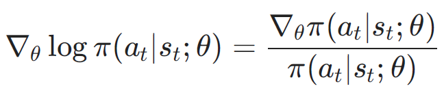
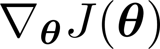
The gradient
rises the log probabilities of the good trajectories
lowers the log probabilities of the bad trajectories
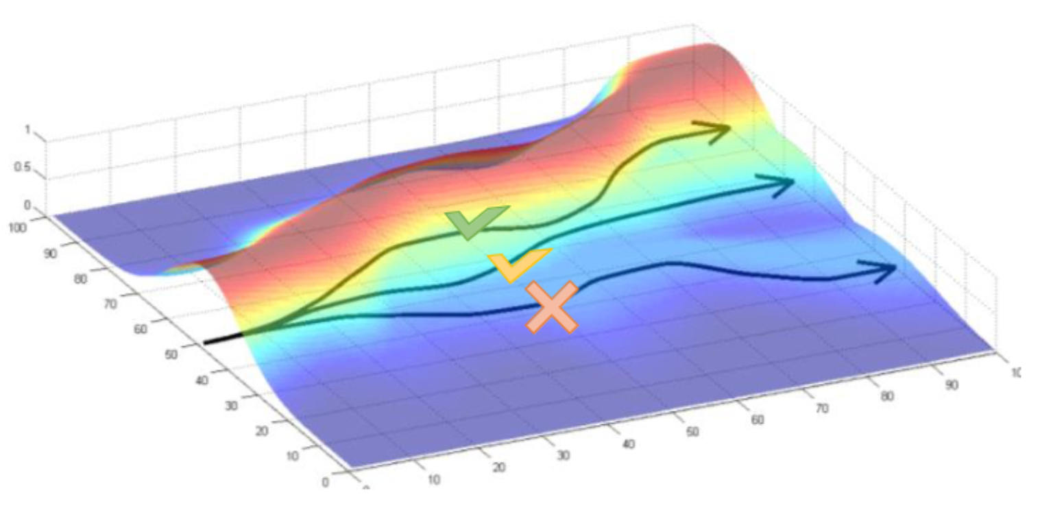
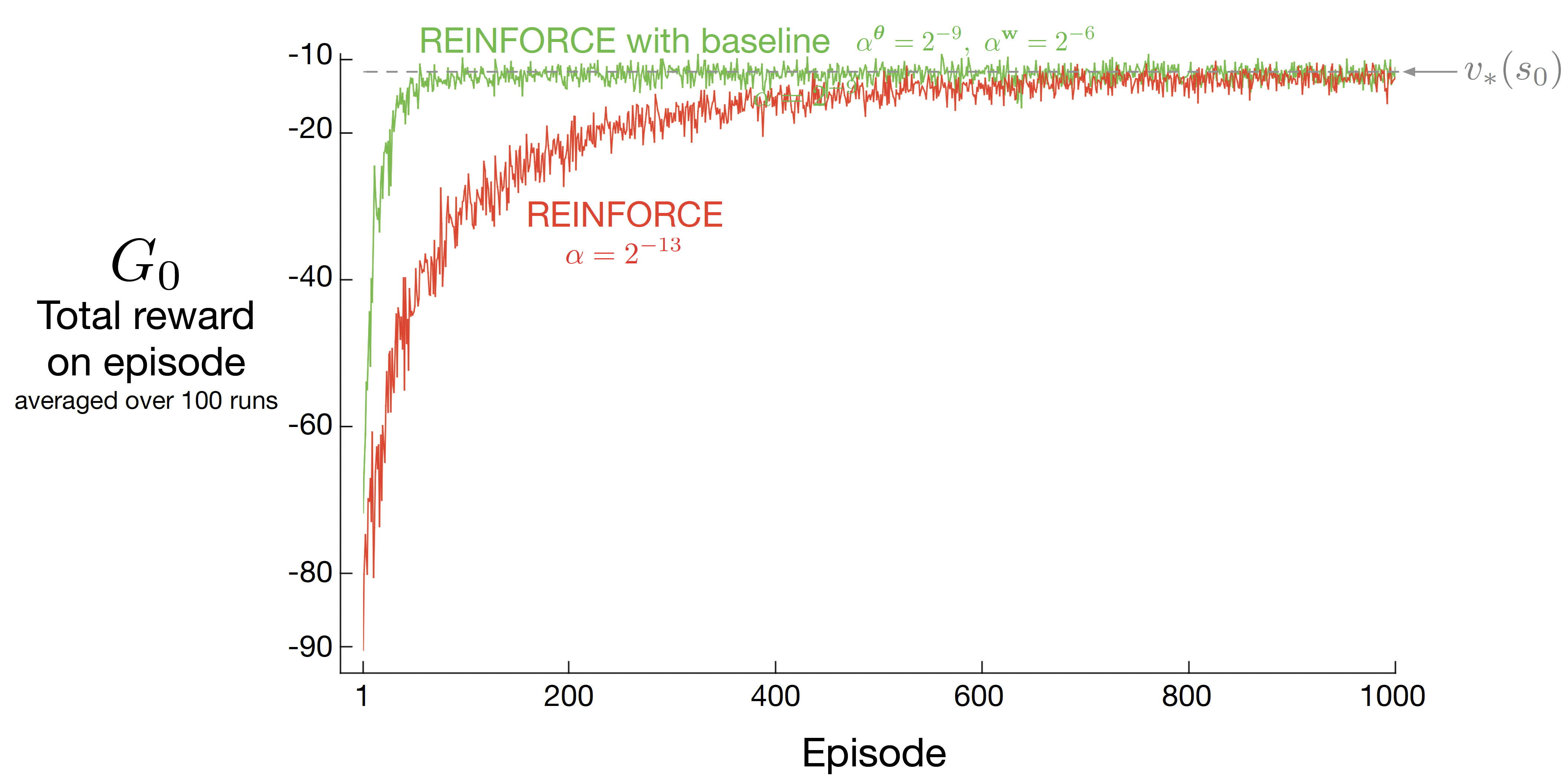
Reducing the variance: Baseline
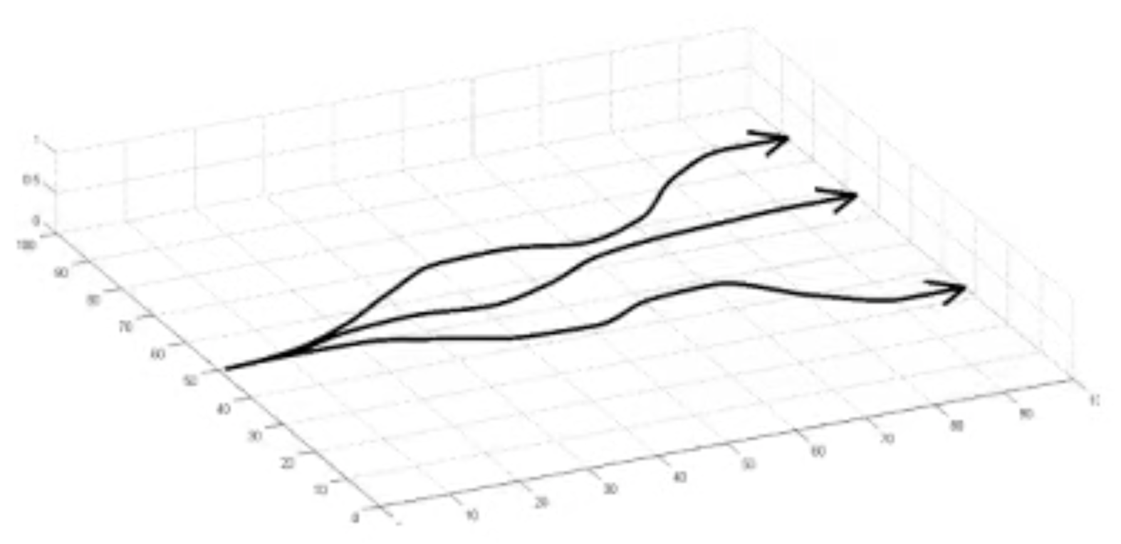
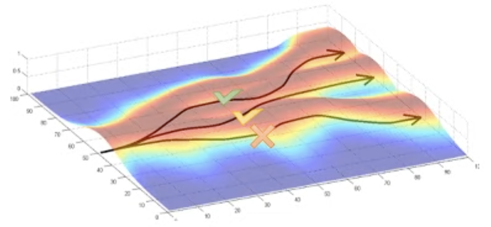
Without Baseline
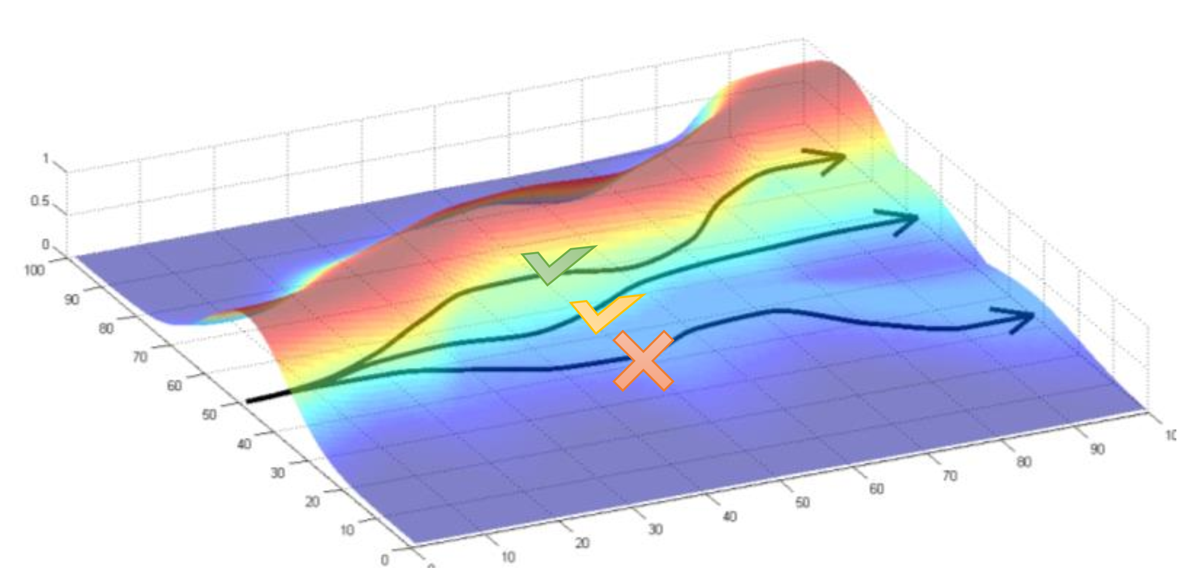
With Baseline
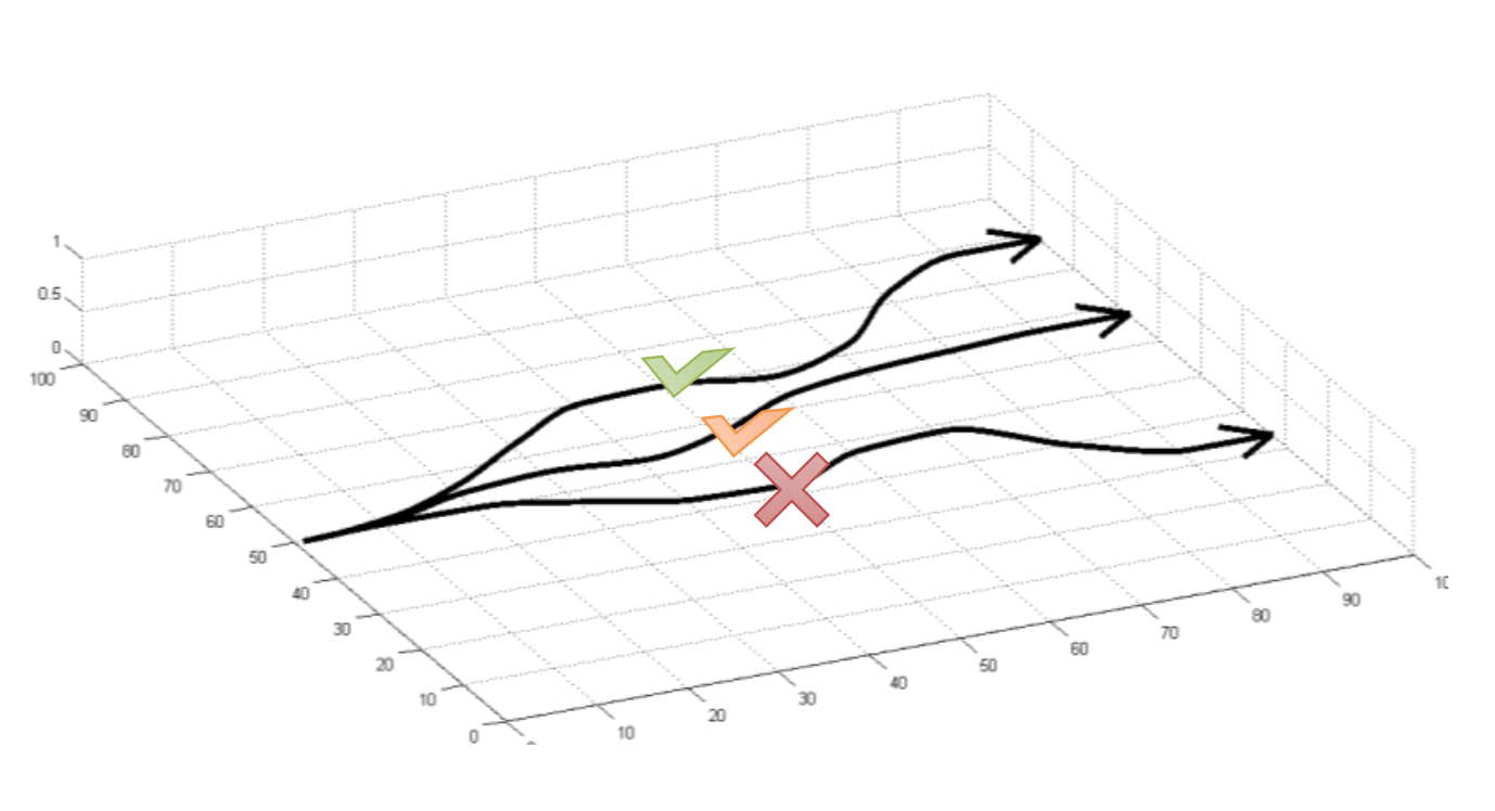
All positive
Subtracting a baseline independent from the action.

![\begin{align*}
\nabla_\theta J(\theta) = \mathbb{E}_{\tau\sim p_\theta(\tau)}\Big[\nabla_\theta \log p_\theta(\tau)(G_t(\tau) - b)\Big]
\end{align*}](media/47ad4625fb.png)
If is , this choice of baselines motivates the Actor-Critic family of algorithms.
Learn the value function via:
MC -> REINFORCE with baseline
TD-learning -> Actor-Critic
Actor-Critic algorithms
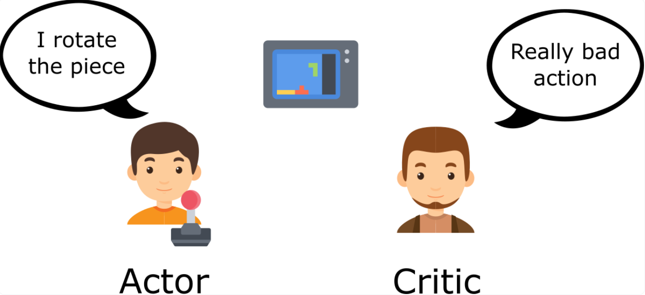
A policy that controls
how our agent acts.
A value function that
measures how good
is the action taken.
Value-Based
Policy-Based
DQN
REINFORCE
Actor-Critic
A2C
Critic
Actor

Policy gradient step
Return

REINFORCE
Estimate the relative improvement of
action at state . Low variance.

![\begin{align*}
\textit{Actor-Critic:}\quad \nabla_\theta J(\pi_\theta) &= \mathbb{E}_t\big[A_t^{\pi}\nabla_\theta \log \pi_\theta(a_t \mid s_t)\big] \\ \textit{REINFORCE:}\quad \nabla_\theta J(\pi_\theta) &= \mathbb{E}_t\big[R_t(\tau)\nabla_\theta \log \pi_\theta(a_t \mid s_t)\big]
\end{align*}](media/074b1ed676.png)
A2C
Advantage
Learns parametrized policy .
Block Diagram of A2C algorithm


Time Difference (TD) error
Recall the advantage function
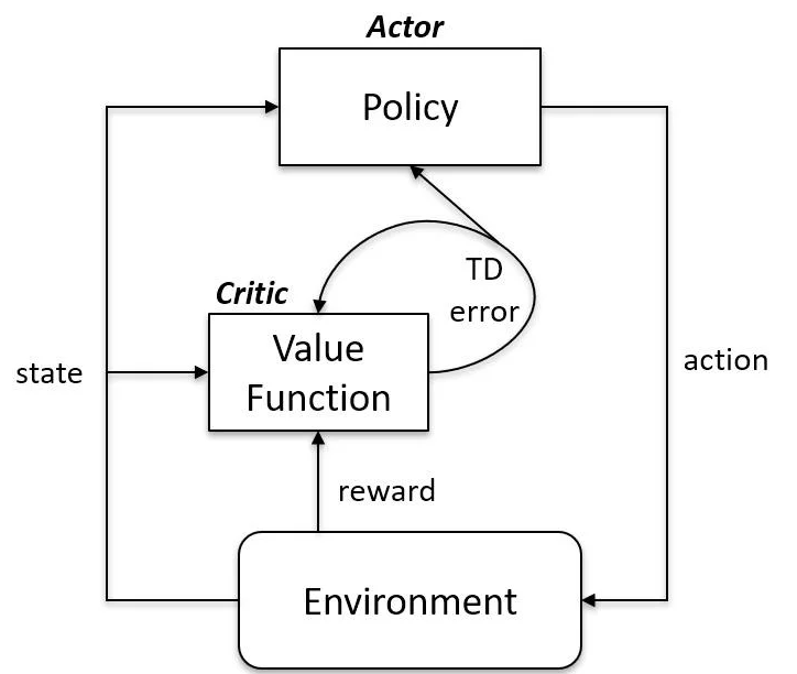
Mnih, Volodymyr, et al. "Asynchronous methods for deep reinforcement learning." International conference on machine learning. PMLR, 2016.
Agent


Policy gradient algorithms (REINFORCE)
•Suitable for continuous state and action space.
•High variance.


Value based algorithms
•Not suitable for continuous action space.
Summary on policy gradient algorithms
Actor-Critic algorithm
•Suitable for continuous state and action space.
•Low variance.
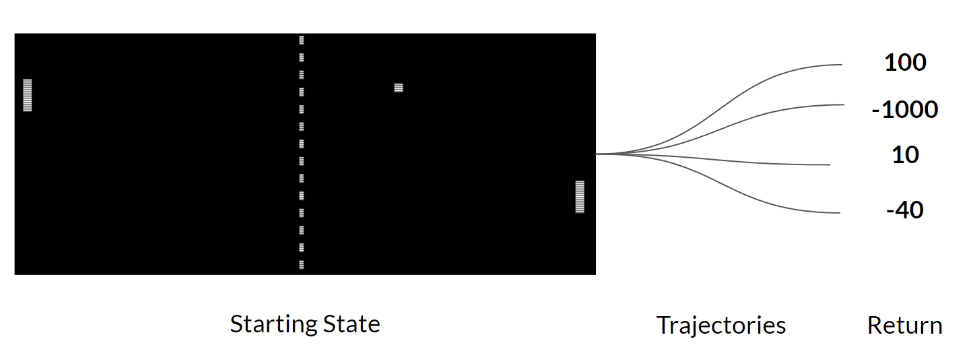

•Model-Free RL
•No Model
•Learn value function (and/or policy) from experience
•Algorithms
•SARSA, Q-learning, REINFORCE, One-step actor-critic, etc.
•Model-Based RL
•Learn a model from experience
•Plan value function (and/or policy) from model
•Algorithms
•Dyna, Monte-Carlo tree search
Today’s lecture
Model-Based RL
Model-Free RL
value functions
experience
acting
learning
Model-Based RL
value functions
experience
acting
learning
model
planning
Model-Based RL
value functions
experience
acting
learning
model
planning
learning
Model-Based vs Model-free RL
value functions
experience
acting
learning
model
planning
learning
value functions
experience
acting
learning
approximation
error
approximation
error
approximation
error
Model-Based vs Model-free RL
value functions
experience
acting
learning
model
planning
learning
value functions
experience
acting
learning
much faster /
data efficiency
supervised learning
methods
More data efficient
No interaction with
the environment
interaction with the
environment make it slower
Reason about
model uncertainty
(better
exploration?)
uses less
often

Model
MDP
Environment
We need to approximate this function!


set of weights


Model
MDP
Environment
We need to approximate this function!


set of weights
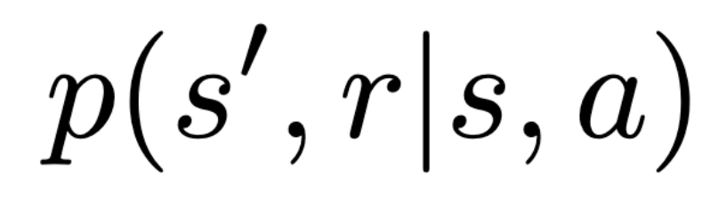
How to estimate this model?
Estimate from experience!
, , …, }
This is a supervised learning problem
,
,
.
.
.
over a dataset of state transitions
observed in the environment.
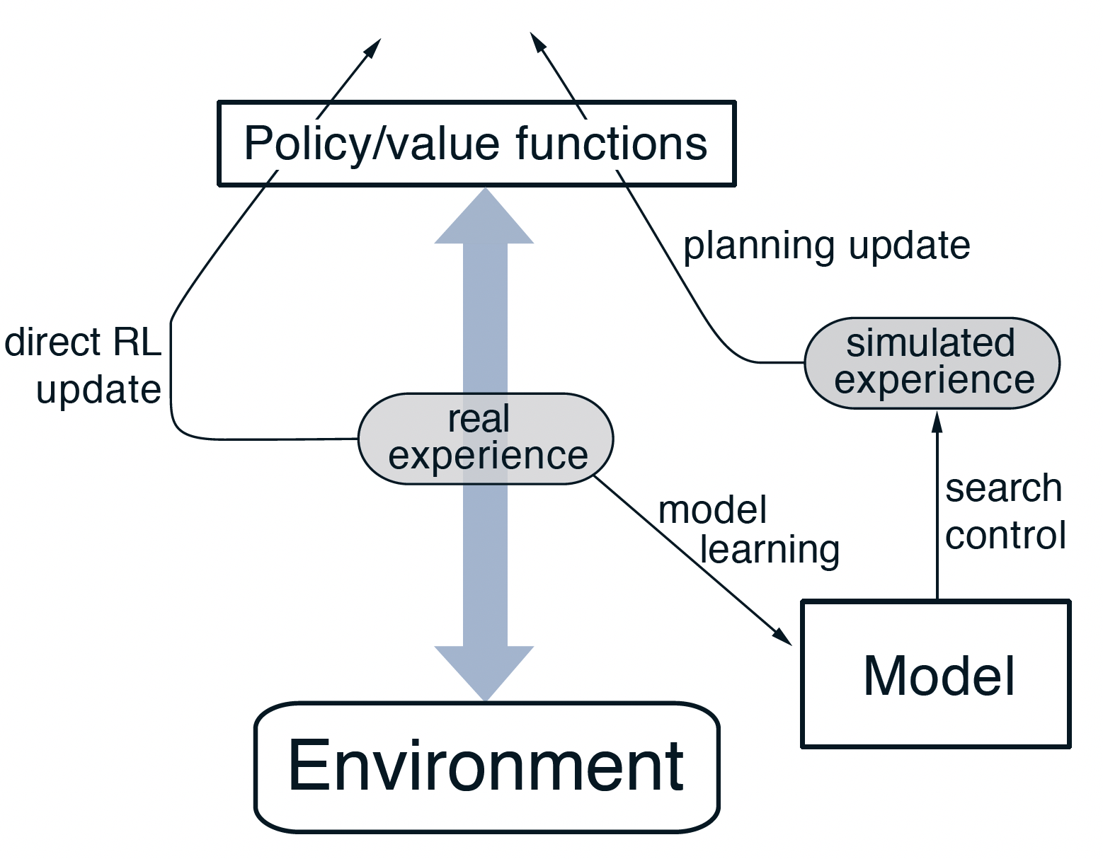
Real and Simulated Experience
Real experience
Sampled from environment (true MDP)
Simulated experience
Sampled from model (approximate MDP)
(planning)
Using learned Model

Solve the approximated MDP
Using dynamic programming
➢Value iteration
➢Policy iteration
Use model to generate samples
➢Monte-Carlo control
➢SARSA
➢Q-learning

Example: Batch Learning in Two States
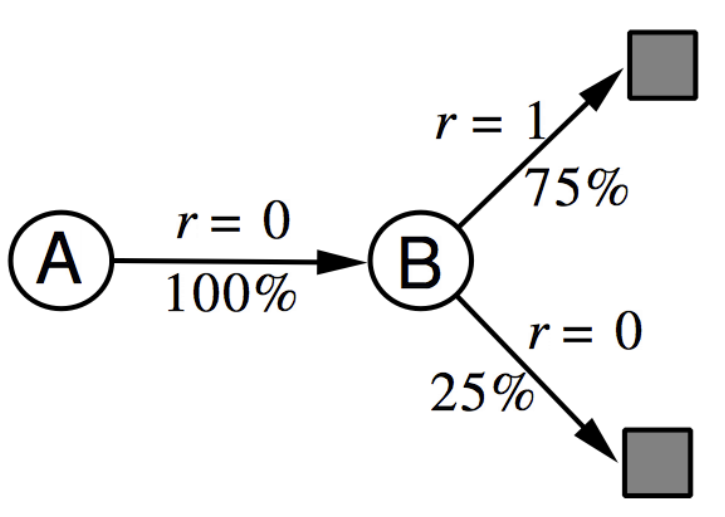
1)A, 0, B, 0
2)B, 1
3)B, 1
4)B, 1
5)B, 1
6)B, 1
7)B, 1
8)B, 0
This is a model!
Monte-Carlo: v(A)=0, v(B)=3/4
Simulated experience
1)B, 1
2)B, 0
3)B, 1
4)A, 0, B, 1
5)B, 1
6)A, 0, B, 1
7)B, 1
8)B, 0
Monte-Carlo: v(A)=1, v(B)=3/4
Real experience
Combined
Monte-Carlo: v(A)=2/3, v(B)=3/4
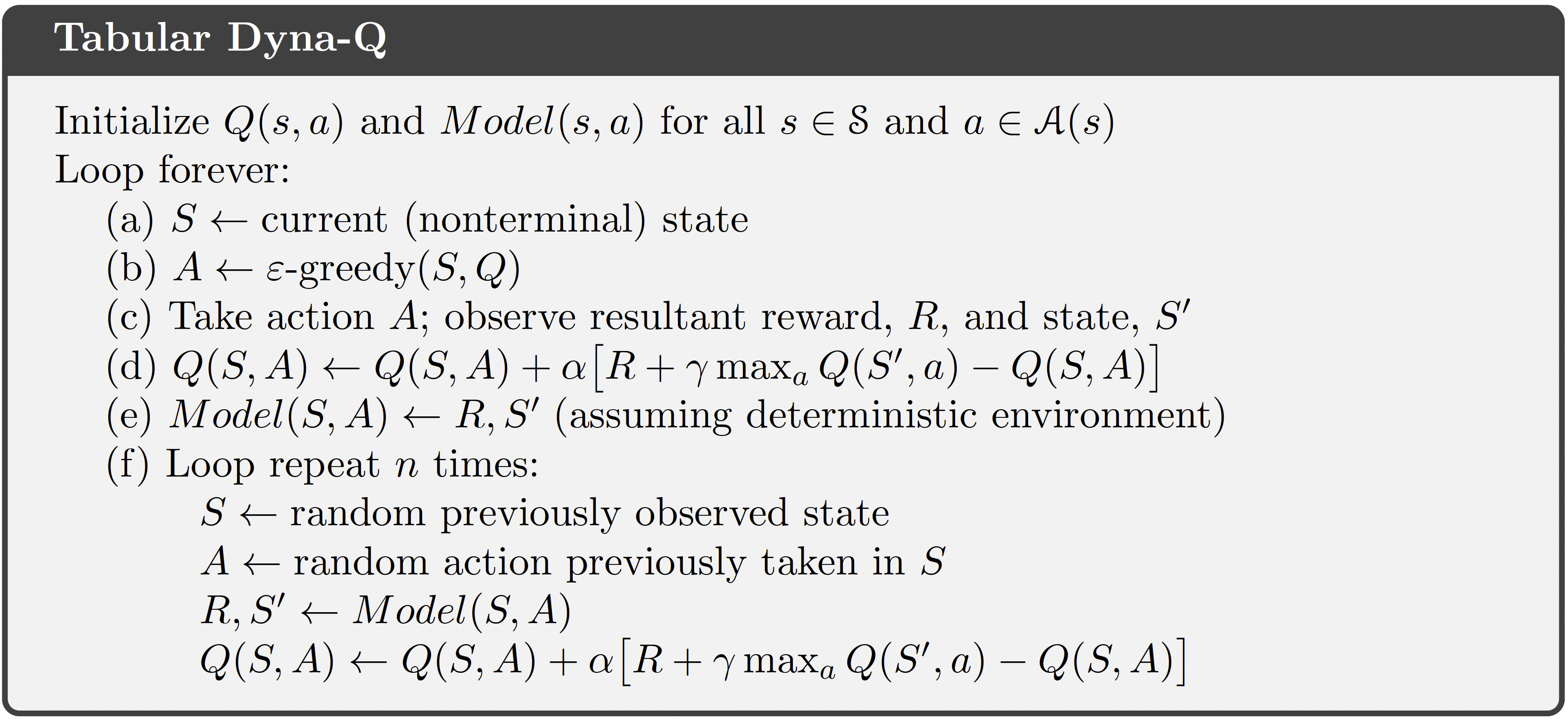
Dyna-Q
Any examples where simulated
experiences are useful?
Robotics
Autonomous driving
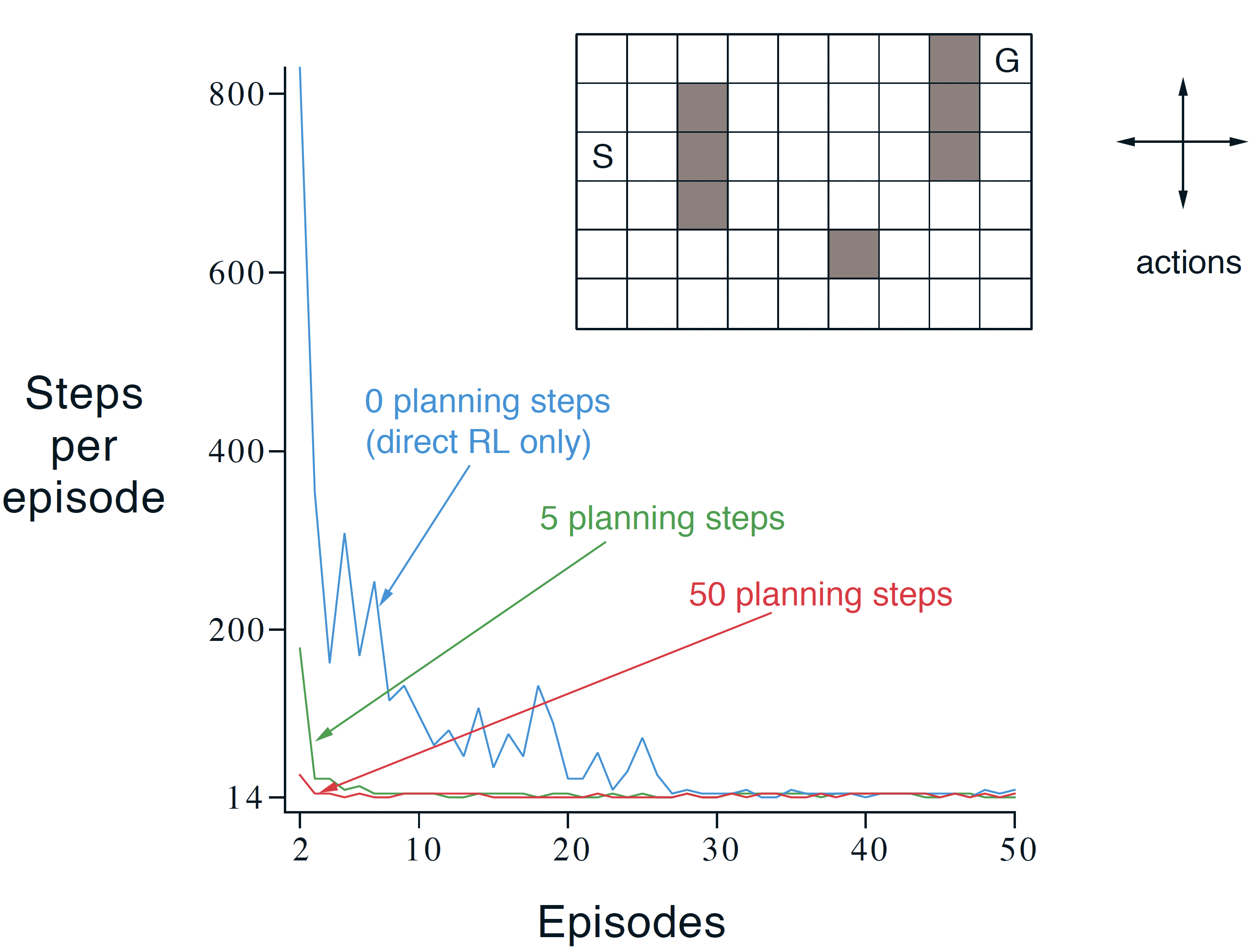
Example: Simple Maze
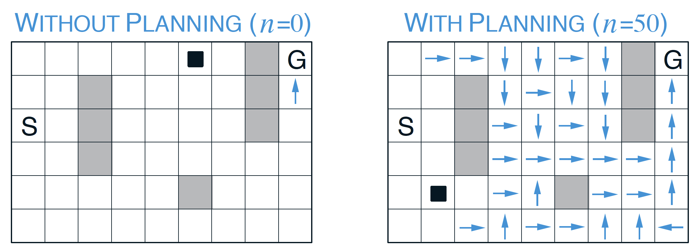
Example: Simple Maze

Dyna-Q with an Inaccurate Model
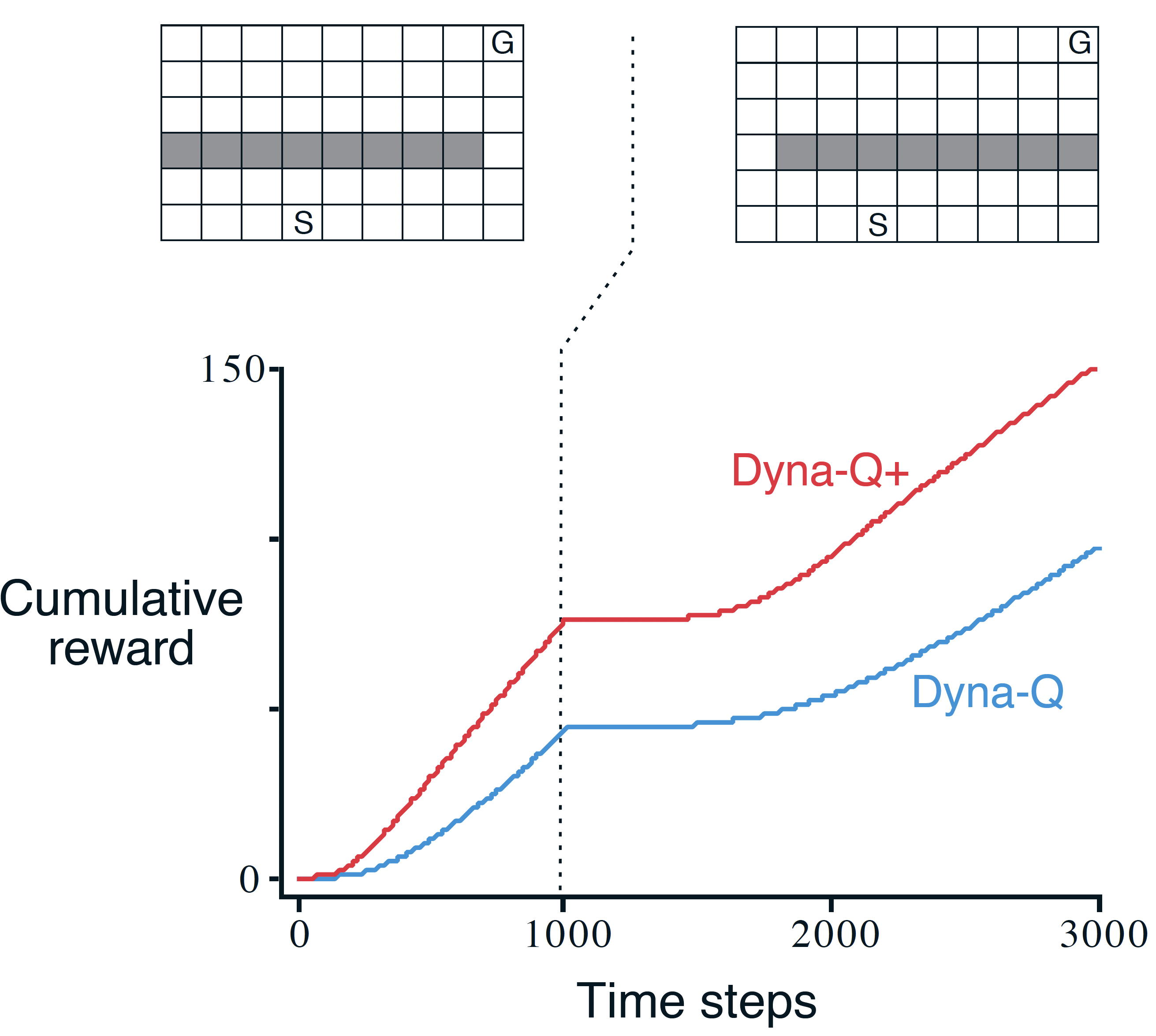
The changed environment is harder
It keeps track for each state-
action pair how many time steps
have elapsed since the pair was
last tried in a real interaction
with the environment.
Dyna-Q with an Inaccurate Model
The changed environment is easier
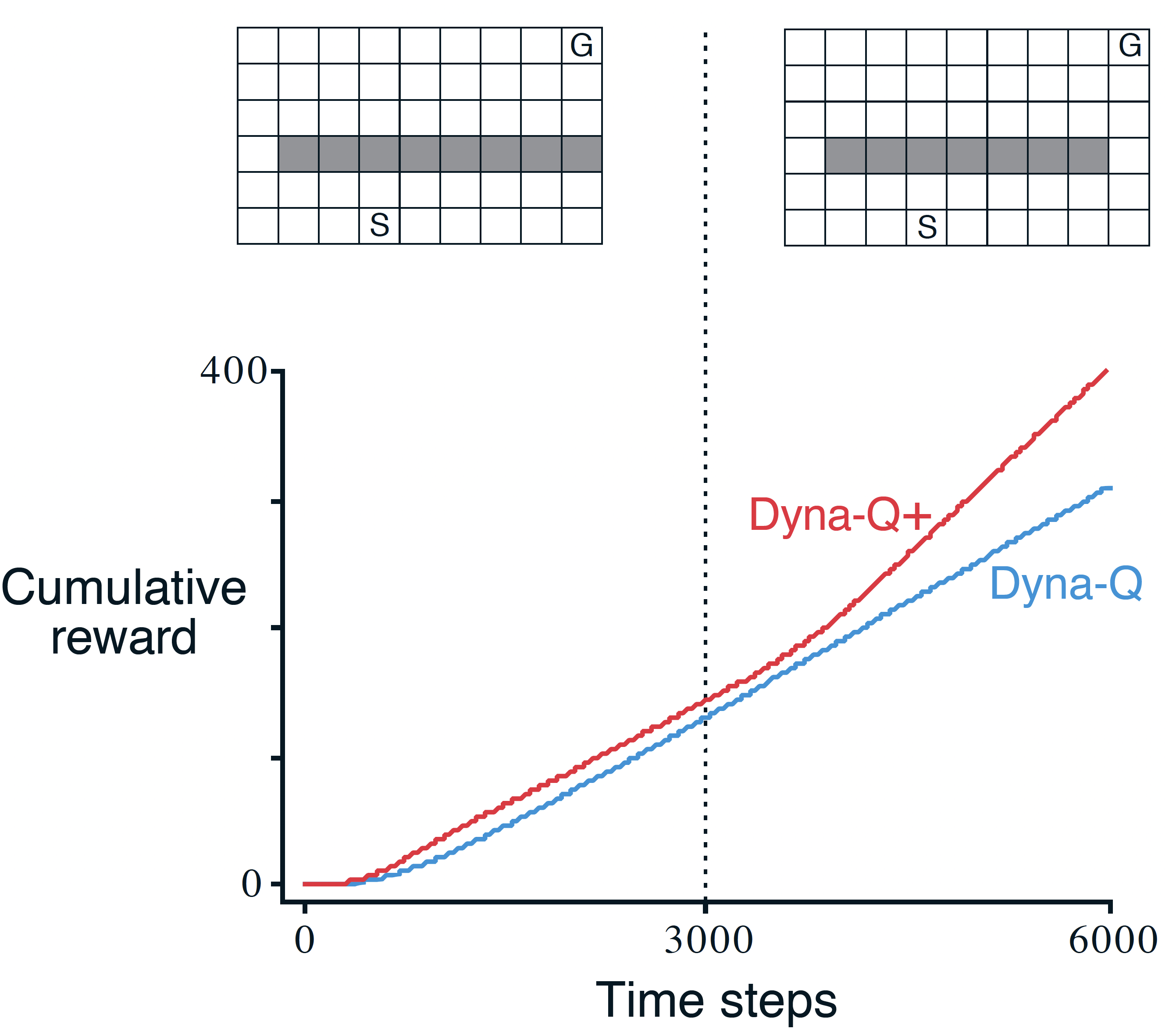
Planning with an Inaccurate Model
•Given an imperfect model
➢The planning process may compute a suboptimal policy
➢Performance is limited to optimal policy for approximate MDP
➢Model-based RL is only as good as the estimated model
•Dealing with the inaccuracies of the learned model
➢Model is wrong => Use model-free RL
➢Reason about model uncertainty over the weights
➢Combine model-based and model-free methods in a single algorithm
Planning and Experience Replay
•Traditional RL algorithms
➢Model-free methods update the value function and/or policy and do not have explicit dynamics
models.
➢Model-based methods update the transition and reward models, and compute a value function or
policy from the model.
Beyond model-based and model-free labels
The sharp distinction between model-based and model-free is now less useful:
1.Often agents store transitions in an experience replay buffer
2.Model-free RL is then applied to experience sampled from the replay buffer
3.Dyna, with the experience replay as a non-parametric model
➢Plan: sampling an entire transition instead of only and inferring from the model
➢Learn: Make it more efficient by making many updates on past data for every new interaction with
the environment.
Planning for Action Selection
•Using planning to improve a global value function
•Planning in the near future to select the action
➢Distribution of states that may be encountered from now can differ from the distribution
encountered from a starting state.
➢The agent may be able to make a more accurate local value function than the global one.
➢Inaccuracies in the model may help exploration.
Forward Search Algorithms

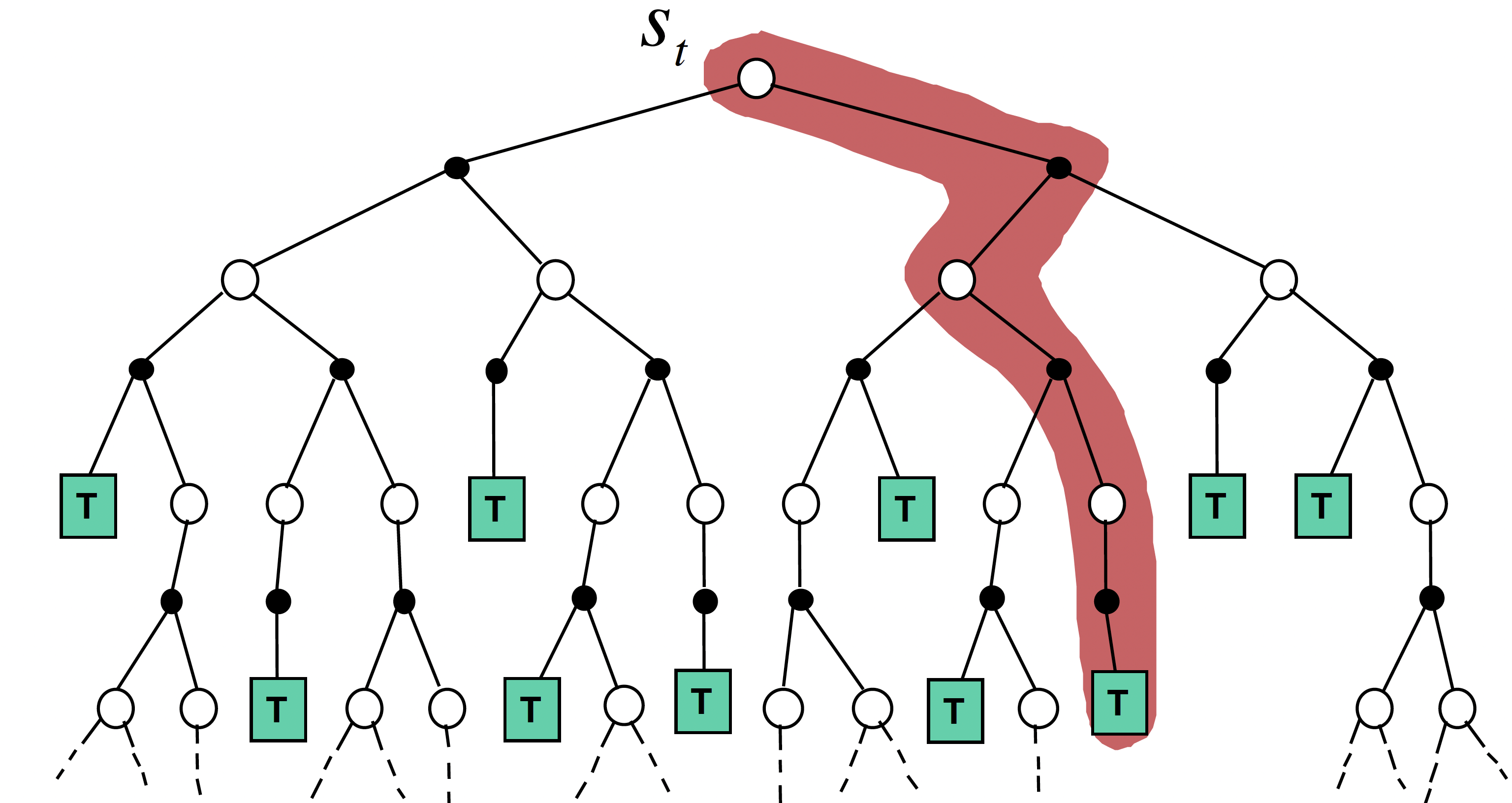
Select the best action by lookahead
build a search tree with the
current state at the root
Using Model of the MDP to look ahead
Forward Search Algorithms

Select the best action by lookahead
build a search tree with the
current state at the root
Using Model of the MDP to look ahead
Only solve sub-MDP starting from now!
Analogy: It’s similar to policy improvement via dynamic programming.
Simulation-Based Search
Sample-based variant of Forward search
Simulate episodes of experience from now with the model
Apply model-free RL to simulated episodes
Analogy: It’s closer to Monte Carlo methods.
Monte Carlo Tree Search (MCTS)
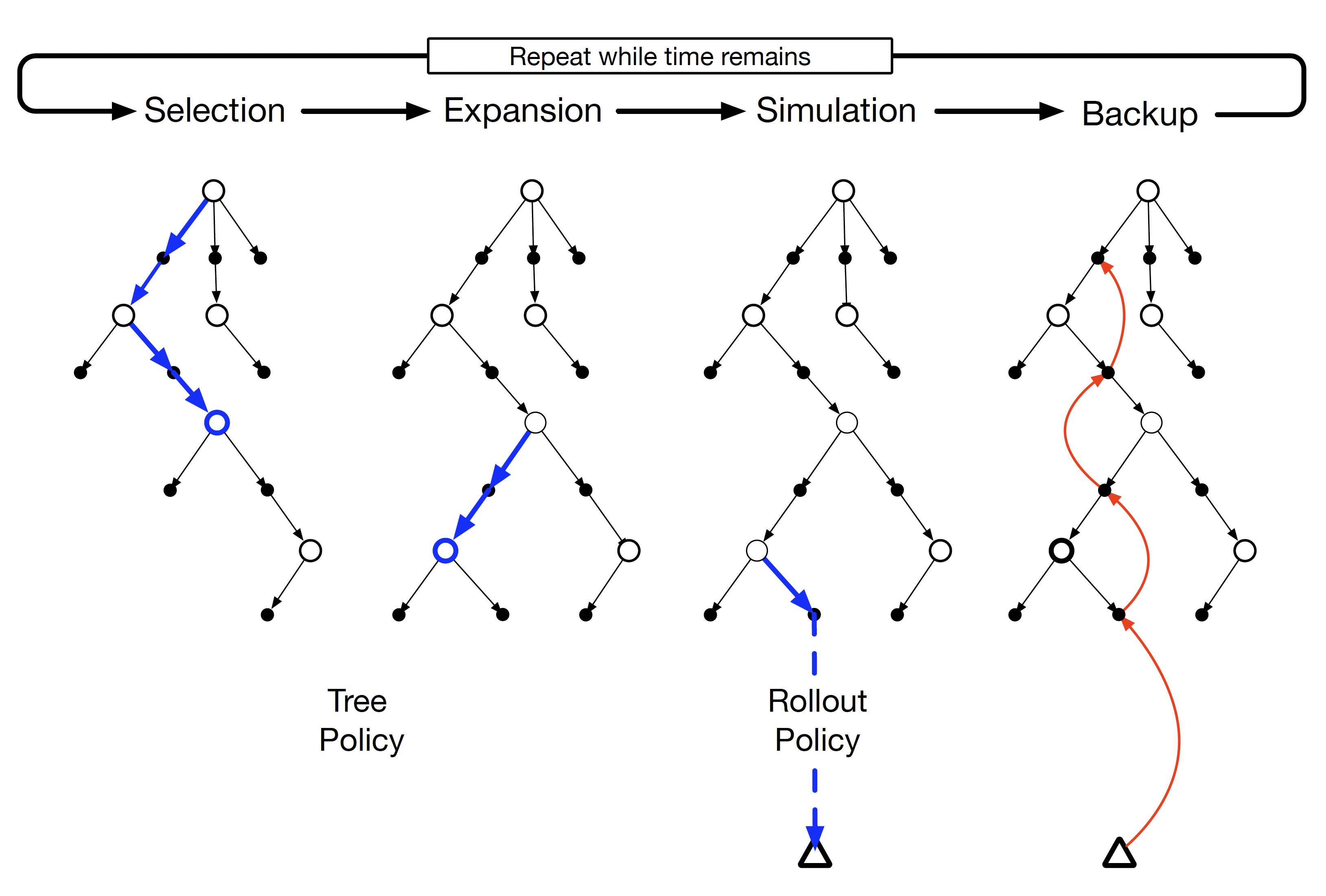
Selected state
(node)
Tree Policy
➢Decide which action to explore next (e.g., using UCT = Upper Confidence bound applied to Trees).
➢Balances exploration vs. exploitation during tree expansion.
➢Depends on the current search statistics (visit counts, value estimates).
Monte Carlo Tree Search (MCTS)

Selected state
(node)
Expanded region
Monte Carlo Tree Search (MCTS)

Rollout Policy
➢Used outside the tree, once a leaf node is
reached.
➢Generates simulated trajectories until
termination (or a depth limit).
➢Usually, a simple heuristic or random policy,
since we can’t afford to plan deeply
everywhere.
Monte Carlo Tree Search

Output: Best action according to in the root node when time runs out.
Advantages of Monte-Carlo Tree Search
➢Highly selective best-first search
➢Evaluates states dynamically (unlike e.g. DP)
➢Uses sampling to break curse of dimensionality
➢Works for “black-box” models (only requires samples)
➢Computationally efficient, anytime, parallelizable
D Silver et al. Nature 529, 484–489 (2016) doi:10.1038/nature16961
Neural network training pipeline and architecture
Example: AlphaGo
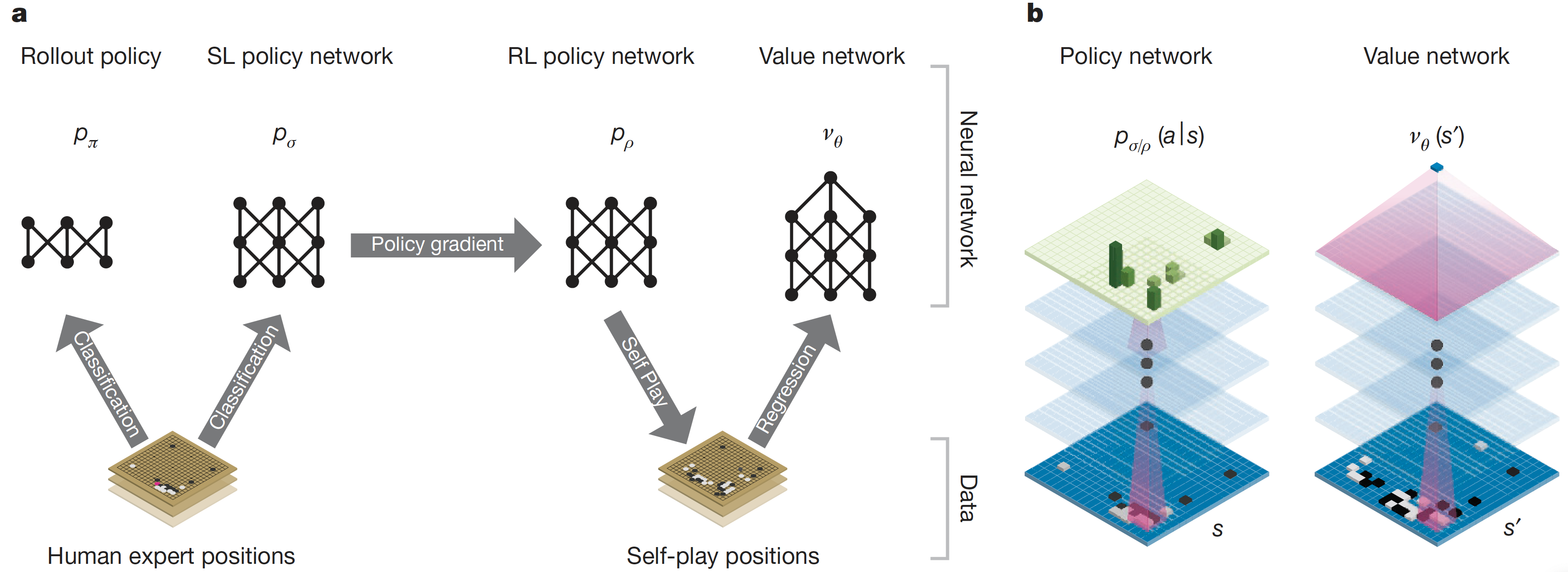
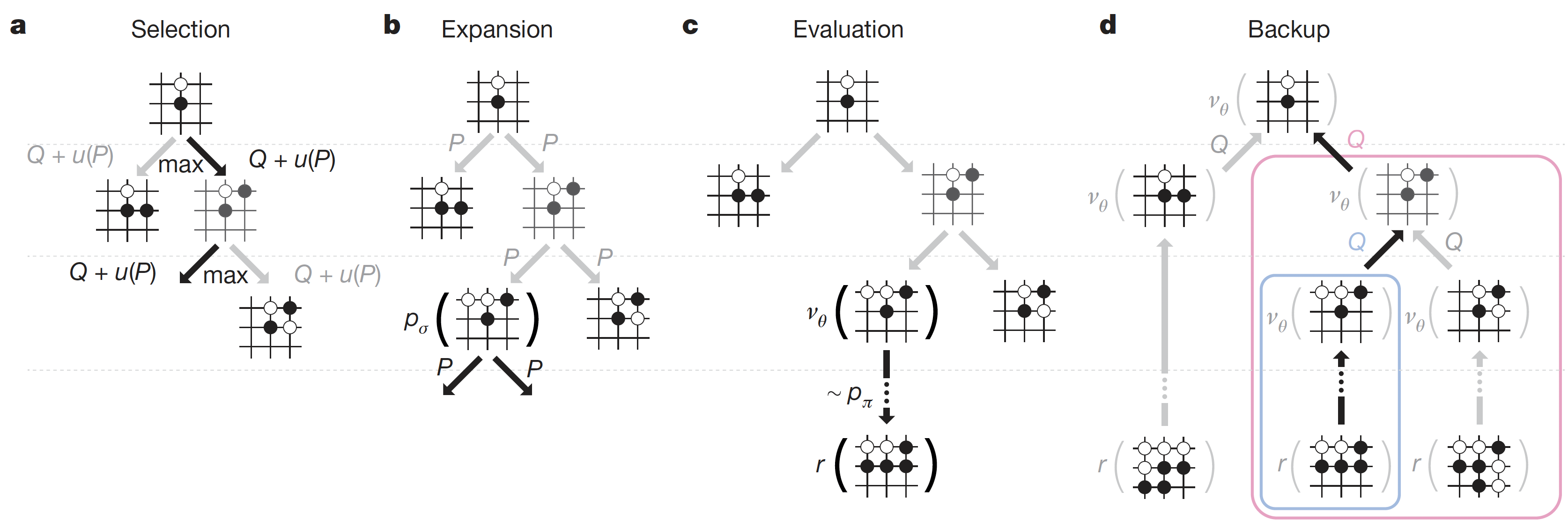
Monte Carlo tree search in AlphaGo
Example: AlphaGo
D Silver et al. Nature 529, 484–489 (2016) doi:10.1038/nature16961
Example: MuZero
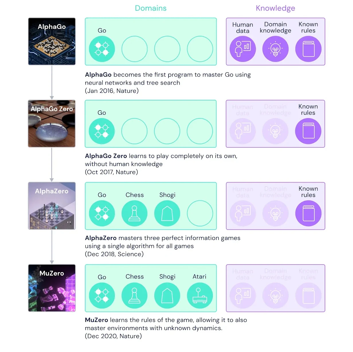
Model-Based RL
•Dyna-Q
•Forward search algorithms
•Monte Carlo tree search
Take home message
•Model-based RL can be
•More data efficient
•But has more approximations susceptible for errors
•The Dyna-q algorithm learns faster in some environments when compared with
model-free RL
•A mix of model-free and model-based RL might improve algorithm performance
Take home message
•Further studying:
•Chapter 8 – Reinforcement Learning: An introduction
•Video (UCL x DeepMind)
•Lecture 8:
https://www.youtube.com/watch?v=FKl8kM4finE&list=PLqYmG7hTraZDVH599EItlEWsUOsJbAodm&in
dex=8