Exercise 5.6.1
Cliff Walking: SARSA, Q-learning, double Q-learning, DQN experiments
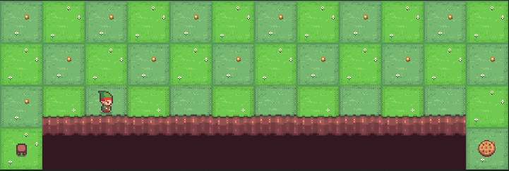
For this question, we are interested in comparing different TD learning methods by running simulations on an environment. The environment in question is the “Cliff Walking“ environment from the Gymnasium library (see also example 6.6 of the book). Cliff-walking has a discrete state and action space, so tabular RL algorithms can be used. Figure 1 shows a visualization of the environment. The goal of the agent is simply to go from the starting point (bottom-left) to the goal (bottom-right) without falling into one of the cliffs. Each time step incurs a -1 reward unless the player steps into the cliff, which incurs a -100 reward. Transitions are deterministic.
The code runs in two workspaces: part (a) in the code workspace, in your browser, and part (b), DQN, in the DQN workspace on a free mybinder.org server. Both have the skeleton project (rl-assignment5); the training loop of its main.py is there for you to use.
-
(a) SARSA, Q-learning, and double Q-learning
1. Implementation: Implement the SARSA, Q-learning, and double Q-learning tabular TD algorithms. The skeleton already has these algorithms inherited from the
TabularAgentclass. You should implement theupdate,behavior_policy, andtarget_policymethods of each algorithm. Note that for SARSA, the behavioral policy is equal to the target policy.-
2. Training and Evaluation: Consider \(\epsilon=0.1\).
Report the learning rate used for each algorithm. Select a number of training episodes that ensures convergence for all three algorithms. Provide two plots: one for the behavior policy and another for the target policy, each plot displaying results for all three algorithms.
Include a caption for each plot, similar to the example provided in the first assignment. To assist with the plots, a
MetricsTrackerobject is provided in the code to keep track of the average return and variance across runs for both the behavior and target policies usingmetric_tracker.record_metric("return", agent_id, episode_idx, value).
-
(b) Train the DQN algorithm from the Stable Baselines3 library on the environment by completing the
train_dqnfunction. When creating the model, select appropriate learning_rate, target_update_interval, buffer_size, and total_timesteps. Report the values you choose. See the DQN documentation on how to do this. Provide two plots: one for the behavior policy and another for the target policy. Include a caption for each plot. To keep track of the cumulative average return with variance, pass theMetricsTrackers to aOffPolicyMetricsTrackerCallbackand give the callback to DQN’slearnmethod. This will ensure therecord_metricmethod is called for the return during DQN training. -
(c) Training results interpretation.
-
1. Provide a theoretical motivation for each algorithm, focusing on speed of convergence, stability, and the maximum return obtained from the behavior and target policy learning curves.
-
2. Explain how you calibrated the learning rate \(\alpha\) for each algorithm.
-
3. For the “Cliff-walking”environment, which algorithm do you consider to be the most data-efficient? Justify your answer.
-
Adapted from Sutton & Barto (2018), Reinforcement Learning: An Introduction, 2nd ed., Example 6.6. Licensed CC BY-NC-ND 2.0.