Exercise 4.5.2
MC, TD(0) and TD(λ) prediction: implement and compare two policies
The programming parts (a)–(c) run in the code workspace, in your browser. It includes the classes for model-free prediction.
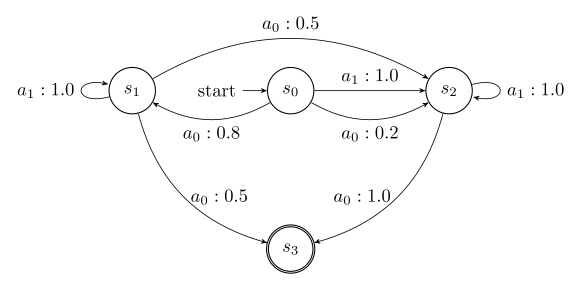
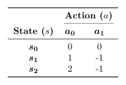
Consider the MDP given in Figure 1. The agent always starts in state \(s_0\). The reward function, which encourages reaching the terminal state \(s_3\), is provided in Table 1. Now, consider the following two policies:
-
Policy \(\pi_1\):
\[\begin{aligned} \pi_1(\cdot |s_0) &=\ a_0 \text{ with probability } 0.70, \ a_1 \text{ with probability } 0.30, \\ \pi_1(\cdot |s_1) &=\ a_0 \text{ with probability } 0.60, \ a_1 \text{ with probability } 0.40, \\ \pi_1(\cdot |s_2) &=\ a_0 \text{ with probability } 0.90, \ a_1 \text{ with probability } 0.10. \\ \end{aligned}\]
Policy \(\pi_2\): \[\begin{aligned} \pi_2(\cdot |s_0) &=\ a_0 \text{ with probability } 0.50, \ a_1 \text{ with probability } 0.50, \\ \pi_2(\cdot |s_1) &=\ a_0 \text{ with probability } 0.30, \ a_1 \text{ with probability } 0.70, \\ \pi_2(\cdot |s_2) &=\ a_0 \text{ with probability } 0.80, \ a_1 \text{ with probability } 0.20. \\ \end{aligned}\]
In the project, the file util/mdp_util.py defines the MDP and \(\pi_1, \pi_2\) for you. The MDP is initialized with a discount factor \(\gamma=0.9\).
We are interested in computing the value function of the two policies. For each of the following algorithms give \(V_{\pi_1} \approx v_{\pi_1}\) and \(V_{\pi_2} \approx v_{\pi_2}\). Use the sample_action method inside the DiscretePolicy class to sample actions for a given state. The MDP class keeps track of a current state and offers reset and step methods. The step method operates similarly to the one in a Gymnasium environment: it expects an action and returns the next state, reward, and whether the next state is terminal.
-
(a) [programming] Implement the MC First-visit prediction algorithms by completing the
_update_value_functionmethod in theMCEvaluatorclass. Run for 1000 episodes. Provide \(V_{\pi_1}\) and \(V_{\pi_2}\). -
(b) [programming] Implement the TD\((0)\) algorithm by completing the
_update_value_functionmethod in theTDEvaluatorclass. Use a step size \(\alpha=0.1\) and run for 1000 episodes. Provide \(V_{\pi_1}\) and \(V_{\pi_2}\). -
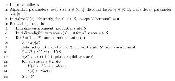
(c) [programming] Implement the TD(\(\lambda\))\(^*\) algorithm by completing the
_update_value_functionmethod in theTDLambdaEvaluatorclass. Use a step size \(\alpha=0.1\), \(\lambda=0.5\) and run for 1000 episodes. Provide \(V_{\pi_1}\) and \(V_{\pi_2}\). -
(d) Using the value function estimates \(V_{\pi_1}, V_{\pi_2}\) show that \(\pi_1 > \pi_2\). Also intuitively explain why this is the case.
*There is a TD(\(\lambda\)) algorithm covered in the book, however that one assumes a differentiable parametric value function approximation. For simplicity we will be focusing on a tabular variant of TD(\(\lambda\)), the pseudo-code code of which is given in algorithm 1. You can see that this formulation is quite similar to TD(0), with the primary difference being the introduction of the eligibility trace. The intuition here is that when a state is visited, its eligibility trace is increased, making it more “eligible” for updates. As time progresses, the traces decay (controlled by the \(\lambda\) parameter), meaning that more recent states have a stronger influence on the updates. Also recall that \(\lambda=0\) is equivalent to TD(0) and \(\lambda=1\) is equivalent to MC.