Exercise 4.4.1
n-step TD: why a 19-state random walk and how n changes with the task
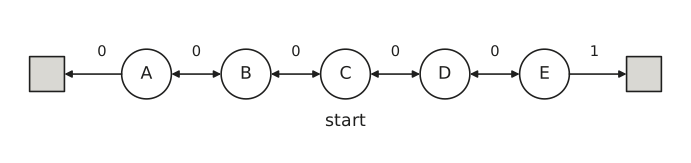
Consider a Random Walk similar to the one in Figure 1 but with \(19\) states. Consider \(n\)-step TD for estimating \(V \approx v_{\pi}\) which uses the following update: \[V_{t+n}(S_t) = V_{t+n-1}(S_t) + \alpha [G_{t:t+n} - V_{t+n-1}(S_t)], \quad 0 \leq t < T\] where \(G_{t:t+n}\) is the \(n\)-step return and \(T\) is the last time step of the episode.
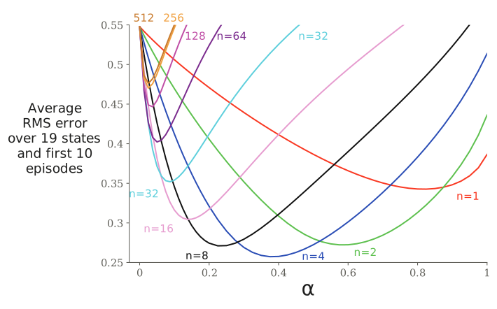
Figure 2 shows the results of a simple empirical test for a larger random walk process, with 19 states instead of 5. The performance measure for each parameter setting, shown on the vertical axis, is the root mean squared error 1 between the predictions at the end of the episode for the 19 states and their true values, then averaged over the first 10 episodes and 100 repetitions of the whole experiment (the same sets of walks were used for all parameter settings).
-
(a) Why do you think a larger random walk task (19 states instead of 5) was used in the Large Random Walk example of Lecture 4?
-
(b) Would a smaller walk have shifted the advantage to a different value of \(n\)?
-
(c) How about the change in left-side outcome from \(0\) to \(-1\) made in the larger walk? Do you think that made any difference in the best value of \(n\)?
Common regression metric (lower = better). For an estimate \(V\) and true value \(v_{\pi}\) the RMSE is \(\sqrt{1 / \mathcal{S} \sum_{s \in \mathcal{S}}(V(s) - v_{\pi}(s))^2}\).↩︎
Source: Sutton & Barto (2018), Reinforcement Learning: An Introduction, 2nd ed., Exercise 7.3; Example 7.1. The random-walk diagram of Example 6.2 is redrawn from the book. Figure 7.2 is redrawn from a new run of the book's experiment. Licensed CC BY-NC-ND 2.0.