Exercise 7.5.4
REINFORCE, actor-critic and PPO: Inverted Pendulum programming task
For this question we are interested in applying the REINFORCE and the one-step actor critic algorithms to the Inverted Pendulum (“InvertedPendulum-v5") environment.
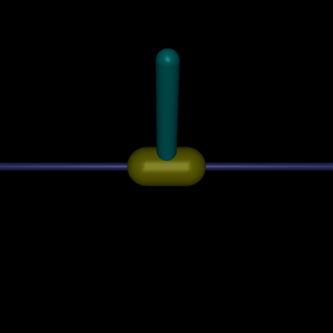
Inverted Pendulum has a continuous state and action space, so advanced RL algorithms like policy gradient methods can be used. Figure 1 shows a visualization of the environment. The goal of the agent is to balance a pole attached to a cart by applying continuous forces between -3 and 3 to the cart. The observation space consists of the cart’s position, the pole’s angle, the cart’s velocity, and the pole’s angular velocity. Each time step incurs a +1 reward as long as the pole remains upright. The environment terminates if the pole falls beyond 0.2 radians.
The code runs in the code workspace, on a free mybinder.org server. It has the skeleton project (rl-assignment6); the training loop of its main.py is there for you to use.
-
a) REINFORCE with baseline and One-Step Actor Critic.
1. Implementation: Implement REINFORCE with baseline and One-Step Actor Critic algorithms. The core algorithm will be implemented in the
ActorCriticAgentandReinforceAgentclasses and you will have to implement the_compute_lossandupdatemethods. The former will compute the objective functions for the policy (the actor) and value function (the critic or baseline) respectively. Theupdatemethod then performs the gradient descent step.-
2. Training and Evaluation: Report the learning rates used for each algorithm. Select a number of training episodes that ensures convergence for all algorithms. Provide a plot for the return across runs.
Include a caption for each plot, similar to the example provided in the first assignment. To assist with the plots, a
MetricsTrackerobject is provided in the code to keep track of the average return and variance across runs.
-
b) Train the PPO algorithm from the Stable Baselines3 library on the Inverted Pendulum environment by completing the
train_ppofunction. When creating the model, select an appropriatelearning_rateandtotal_timesteps(the other hyperparameters can stay at their defaults). Report the values you choose. See the documentation on how to do this. Provide a plot for the return across runs. Include a caption for each plot. To keep track of the average return with variance, pass theMetricsTrackers to aMetricsTrackerCallbackand give the callback to PPO’slearnmethod. -
c) Training results interpretation.
1. Provide a theoretical motivation for each algorithm, focusing on speed of convergence, stability, and the maximum return obtained from the loss and the policy learning curves.
2. Explain how you calibrated the learning rates \(\alpha^{\mathbf{w}}, \alpha^{\theta}\) for each algorithm.
3. For the “Inverted Pendulum” environment, which algorithm do you consider to be the most data-efficient? Justify your answer.
Hints:
For performance evaluation, consider also inspecting the loss/objective curves and see if they go down, look at a recording of the environment. It might also be worth doing an evaluation run and examining the reward curve after the agent has been trained.
PyTorchby default can only do gradient descent. Recall that the policy-gradient objective is optimization using gradient ascent. For that reason you will have to reverse the sign of the objective. This means the ‘policy loss’ will be \(-\ln \pi(A_t|S_t, \theta) \cdot \delta\). Note that the value function parameters are updated using gradient descent so there will not be a sign change there.Make use of the
sample_actionandlog_probmethods of theStochasticPolicyNetworkclass.Use
detach()on the advantage (\(\delta\) in the pseudocode) when computing the policy loss. This is to ensure the gradients from the value function (critic) loss, which is derived from the advantage term, does not backpropagate through the computation of the advantage when updating the policy (actor) parameters. Ensuring the critic’s loss and the actor’s loss are treated as independent in terms of gradient flow.For the gradient update you can add the losses of the actor and the critic and then run the backwards method on the resulting tensor. Do note that we have two optimizers for the actor parameters \(\theta\) and critic parameters \(\mathbf{w}\).
The REINFORCE algorithm pseudocode has a for loop after generating an episode. Since PyTorch can use batch operations you do not need to explicitly make a loop. If you have a batch of input tensor of the shape
(batch_size, dim)and you pass it to a module (e.g., a neural network) expecting a tensor of shape(, dim)and returning a tensor of shape(, out_dim)then you will get a tensor of shape(batch_size, out_dim)containing the output for each batch input.You can add batch updates to the One-Step Actor Critic algorithms by waiting a number of steps before updating and then performing the update on a batch of transitions. This can stabilize the learning slightly but should not be necessary for solving the inverted pendulum environment.
NOTE: Regarding the environment. If the environment has a discrete action space, then our function approximator for the policy can simply output a discrete probability distribution (which gives a probability for each action). In the context of neural networks, this would mean \(n\) output neurons for \(n\) actions with a softmax activation function.
However, the Inverted Pendulum environment has a continuous action space, which we need to take into account when parameterizing the policy. If the action space is (a subset of) \(\mathbb{R}\), then the policy can be defined as a Gaussian probability distribution \(\mathcal{N}\), with mean \(\mu\) and standard deviation \(\sigma\) given by parametric function approximators that depend on the state: \[\pi(a|s, \theta) = \mathcal{N}(a|\mu(s, \theta), \sigma^2(s, \theta)).\] Here \(\mu : \mathcal{S} \times \mathbb{R}^{d} \rightarrow \mathbb{R}\) and \(\sigma : \mathcal{S} \times \mathbb{R}^d \rightarrow \mathbb{R}^+\) are two parameterized function approximators and \(d\) is the feature vector dimensionality.
Instead of using two function approximators, we can use a neural network with two output heads, one for the mean and the other for the standard deviation. We can then get a continuous scalar action for an action by passing the state \(S\) to the neural network, computing the two output heads, constructing the Gaussian distribution, and sampling an action from the Gaussian distribution \(A \sim \mathcal{N}(a|\mu(s, \theta), \sigma^2(s, \theta))\).
Lastly, if we have \(n\)-dimensional continuous actions \(\mathbf{a} \in \mathcal{A} \subseteq \mathbb{R}^n\), then the mean head will output an \(n\)-dimensional mean vector \(\pmb{\mu}\) and the other head an \(n \times n\) covariance matrix \(\mathbf{\Sigma}\) (more precisely, the unique elements of the covariance matrix will be outputted as a vector). The process is otherwise the same with \(A \sim \mathcal{N}(\mathbf{a}| \pmb{\mu}, \mathbf{\Sigma})\).
In the models module of the skeleton code, there is an implementation of a two-headed multilayer perceptron.